Universal time delay in static spherically symmetric spacetimes for null and timelike signals

Today, the time delay of gravitational lensed images by compact objects, galaxies, or their clusters has become an effective tool in astrophysics and cosmology [1]. For lensing by compact objects, the time delay can be used to constrain properties of the spacetime, such as its mass or naked singularities [2, 3]. For galaxies or galaxy clusters, time delay can be used to independently and accurately measure the Hubble parameter to a percentage level, and to constrain the lens mass profile, the line-of-sight mass distribution, dark matter substructures, and the dark Universe parameters [4-10].

Traditionally, the time delay has always been obtained from light spectral data. With the discovery of extragalactic neutrinos [11-14] and gravitational waves (GWs) [15-19], particularly the lensed supernovas [20, 21] and simultaneous observations of GW+GRB events [18, 19], it is clear that both neutrinos and GWs can function as messengers of the time delay effect. Although neutrinos [22] as well as GWs in some gravitational theories beyond GR [23, 24] are known to have nonzero masses, the formulas for null rays were used in previous considerations of their time delays [10, 25-27]. Since the subluminal speed of these massive particles can also contribute to the time delay, timelike geodesics, rather than null ones, should be used for computation if high accuracy is desired.

Previously, we have demonstrated that the time delay in the Schwarzschild spacetime for null or timelike rays receives factors of correction [28]. However, when considering other spacetimes, the effect of the spacetime parameters such as electromagnetic charges, angular momentum, and other effective charges such as in the Bardeen [29, 30], Janis-Newman-Winicour [31], and Einstein-Born-Infeld spacetimes [32, 33] on the time delay is still unclear. In this work, we present a perturbative method of calculating the total travel time and time delay in arbitrary static spherically symmetric (SSS) spacetimes for null and timelike signals with general velocities. The result of the total time takes a quasi-series form of the impact parameter b, and the time delay to the leading order(s) takes a universal form depending on the leading expansion coefficients of two metric functions. We use the geometric unit $G = c = 1$ throughout the letter.

The most general SSS metric can be described by

where $(t,\; r,\; \theta,\; \varphi)$ are the coordinates, and $A,\; B,\; C$ are metric functions depending on r only. It is routine to find the geodesic equations in this metric

in which $\kappa = 0,\; 1$ for null and timelike signals, respectively. Here, L and E are first integral constants representing the angular momentum and energy of the null ray or the unit mass of the timelike particle, respectively. Note that because of the spherical symmetry, we will always set $\theta = \pi/2$ for the geodesic motion without losing any generality. Using Eqs. (3) and (4), we can obtain the equation of motion for ${\rm{d}} t/ {\rm{d}} r$. Further integrating it from the source located at radius $r_s$ to the closest radius $r_0$ and then to a detector at $r_d$, we obtain the total travel time t of the signal:

Note that we have not canceled some terms in the numerator and denominator for later convenience in Eqs. (14) and (15). In this letter, we focus on asymptotically flat spacetimes, in which L and E are related to the velocity v at infinity and impact parameter b by

Although this equation is only valid for massive particles, the relationship

can be used for both null and timelike rays. Indeed, in the deflection angle computations in this paper, taking the $v\to 1$ or $E\to\infty$ limit will always produce results for null rays. The angular momentum L can also be related to $r_0$ using the radial equation of motion ${\rm{d}} r/ {\rm{d}} t|_{r = r_0} = 0$, to determine

Further using Eqs. (6) and (8) for timelike rays and Eqs. (7) and (8) for null rays, we can establish a relationship between the impact parameters b and $r_0$

where, in the final step, we denote $1/b$ as a function p of $1/r_0$.

The key to proceeding is to perform a special change of variables in the total time formula (5), after which we can conduct a series expansion of the impact parameter and subsequently rigorously prove the integrability of the expansion for null and timelike rays in arbitrary SSS spacetimes. The variable change simply utilizes the inverse function of $p(x)$, which we denote as $q(x)$, such that r is changed to u through the relationship

or equivalently

where, in the second step, Eqs. (9) and (10) are used. Now, using Eqs. (11) and (6), the infinitesimal and the first fractional term in the integrand of Eq. (5) respectively become

Using Eqs. (8) and (12), the second fractional term in the integrand of Eq. (5) becomes

Note that, on the right hand sides of Eqs. (14) and (15), q is $q(u/b)$ and $p^\prime$ is the derivative of function p. The integral limits of Eq. (5) should change to the limits of variable u, i.e.,

Collecting these together, the total time (5) becomes

where

Note that this function ${ y( u/ b)}$ depends on u only through the ratio $u/b$. Using definition (18), when the metric functions $A(r),\; B(r)$, and $C(r)$ are known, ${ y( u/ b)}$ can be series expanded in the powers of $u/b$ to yield the result

where $y_n$ denotes the expansion coefficients. Note that the explicit form of the inverse function $q(x)$ is not required in this process since we can use the Lagrange inversion theorem and function $p(x)$ to obtain its expansion. To obtain the general form of $y_n$, we will use the following asymptotic expansion of the metric functions

where $a_n$, $b_n$, and $c_n$ are finite constants. Without losing any generality, the constant $a_1$ will later be identified with the ADM mass M of the spacetime $(a_1 = -2M)$, and the constant $b_1$ is conventionally referred as the $\gamma$ parameter $(b_1 = 2M\gamma)$ in the parameterized post-Newtonian (PPN) formalism of gravity [34]. Substituting these into Eq. (18) and determining the power expansion of $u/b$, the first three orders of $y_n$ are observed to be (see Appendix A for details)

We observe that for the order n coefficient $y_n$, only the coefficients up to order $n+1$ of the metric functions contribute.

Substituting Eq. (19) into the total time (17) and performing a further change of variable $u = \sin\theta$, which is suggested by the denominator $\sqrt{1-u^2}$, this becomes

where we denote, respectively,

Here, the integrability of Eq. (22) to any desired order of $y_n/b^n$ becomes clear because the integration part can always be calculated to yield

and for odd and even positive n, respectively, [35]

Therefore, the total time (22) becomes

where $y_n$ are given in Eq. (21) and $l_n$ in Eqs. (24) and (25). This is the total travel time applicable to all SSS spacetimes and both null and timelike rays, as well as for both large and smaller impact parameters b.

For practical gravitational lensing (GL) observation, the relationship $r_{s,d}\gg b$ is satisfied. Moreover, we will assume that the expansion parameters of the metric functions in Eq. (20) satisfies the weak field limit, i.e., ${\cal{O}}(b^n)\gg |a_n|,\; |b_n|$ or $|c_n|$. In these two limits, we can expand the total time (26) in the powers of $\dfrac{1}{b}$ and $\dfrac{b}{r_{s,d}}$. Therefore, we can expand the first three $l_n$ $(n = -1,0,1)$ in Eqs. (24) and (25) to the order of $\left( \dfrac{M}{b} \right)^1$ and $\left( \dfrac{b}{r_{s,d}} \right)^1$

Substituting this expansion and Eq. (21) into Eq. (26), the total time becomes

where all terms are arranged in a decreasing order. The first, second, and fourth terms, i.e., the ${\cal{O}}(r_i)$, ${\cal{O}}(b^2/r_i)$, and ${\cal{O}}(M)$ order terms, are obtained from $l_{-1}$ in Eq. (27). Similarly, the third and part of the sixth terms, which are of orders ${\cal{O}}(\ln(r_i/b))$ and ${\cal{O}}(M^2/r_i)$, respectively, originate from $l_0$. The fifth and remainder of the sixth terms, of orders ${\cal{O}}(M^2/b)$ and ${\cal{O}}(M^2/r_i)$, originate from $l_1$. As we will demonstrate next, expansion to these orders is sufficient to determine leading order(s) useful for observations. In Ref. [36], the total travel time for null rays were also computed using PPN parameters. We have compared our result (28) with their Eq. (3.4) and observed that at orders ${\cal{O}}(r_i),\; {\cal{O}}(b^2/r_i),\; {\cal{O}}(M\ln(r_i/b)),\; {\cal{O}}(M)$, our results agree analytically. For even higher order results, i.e., ${\cal{O}}(M^2/b),\; {\cal{O}}(M^2/r_i)$, owing to the different approximations used, our results are only consistent at the magnitude level. However as we will discuss in Sec. III, these higher order terms will not contribute to the leading order result of the time delay.

Using the total time (28), we can compute the time delay between images of the same source in GL. For this, we first must determine the total time of each image separately. Let us assume that the source, lens, and detector are in the configuration depicted in Fig. 1, where $\phi_0$ is the angle of the lens-source direction against the lens-detector axis. $\beta$ denotes the angle of the detector-source direction against the lens-detector axis in the no lens limit. Using triangles $\triangle ASL$ and $\triangle ASD$, apparently we can establish the geometric relation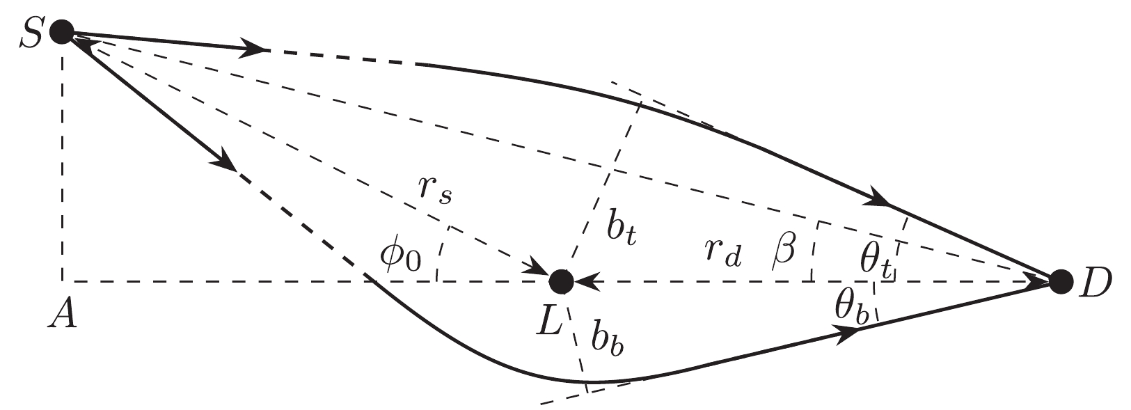

Figure 1.  The GL in an SSS spacetime. $S,\; L,\; D$ are the source, lens, and detectors. $b_b$ and $b_t$ are the impact parameters for the bottom and top paths, respectively. For this configuration with small but positive $\phi_0$ (or $\beta$), $b_t>b_b$ as can be seen from Eq. (32), and consequently, the flight time from the top will be shorter, as dictated by Eq. (28).

between the two angles $\phi_0$ and $\beta$ and the source and detector radii $r_s$ and $r_d$, respectively.

Thus, for the two paths of any given two images, the only parameter that is different in the total time formula (28) or (26) is their impact parameter b. Therefore, we must devise a means of comparing these two b's to compute their time delays. Here, we avoid as much as possible any non-exact equations or equations whose truncation errors are difficult to track, such as the approximate equation $b\approx r_d \theta$ where $\theta$ is the apparent angle of the images. Rather, in this letter, we use a more exact and trackable method to link the two impact parameters.

From Ref. [37], the change of the angular coordinates $\Delta \varphi$ from the source to the detector in an SSS spacetime has been computed as a series form to high order of $M/b$. For the purpose of time delay, we will only use this series to the first order of $M/b$ and $b/r_{s,d}$ (henceforth we use M and $\gamma$ to completely replace $a_1$ and $b_1$), i.e.,

We emphasize that to this order, among all expansion coefficients in Eq. (20), $\Delta \varphi(b)$ only depends on mass M and $\gamma$ but not high order $a_n,\; b_n\; (n = 2,\cdots)$ or any of $c_n\; (n = 1,2,\cdots)$. One will see later that this point contributes to the universality of the time delay to the leading order(s) in Eq. (38).

For GL shown in Fig. 1, the change of the angular coordinates from the bottom and top sides are respectively $\pm \pi + \phi_0$. Equating them to Eq. (30) with b substituted by impact parameters $b_{t,b}$ from both sides, we have

where the sign on the top (or bottom) is for the top (or bottom) path. From this, we can solve $b_{t,b}$ as

where

Equation (32) establishes a simple and yet accurate relation between the angle $\phi_0$ and the impact parameters, with the only approximation tracking back to the truncation of the change in the angular coordinate (30). Since $\phi_0$ is small and positive, it is clear from Eq. (32) that $\eta>0$ and therefore the impact parameter $b_t$ of the signal from the same side of the source against the lens-observer axis will be larger than $b_b$, the impact parameters of the signal from the other side.

Substituting these two impact parameters (32) and $a_1 = -2M$ into the total time (28), we see from the leading relevant term $-b^2/(r_iv^2)$ that the flight time of the top trajectory with a larger impact parameter $b_b$ will be smaller than that of the bottom trajectory with a smaller impact parameter $b_t$. Subtracting each other, we see that the leading, fourth, and sixth terms of Eq. (28), i.e., the ${\cal{O}}(r_i),\; {\cal{O}}(M)$, and ${\cal{O}}(M^2/r_i)$ order terms, are exactly canceled between the two total times. The second, third, and fifth terms, which emerged as the respective leading terms in the expansion of $l_{-1},\; l_0$, and $l_1$ in Eq. (27), become respectively the three terms in the following result for the time delay:

It is then easy to see that when

the logarithmic term of Eq. (34) will take a form of $\ln(1+\text{ a small quantity})$ and a Taylor expansion can demonstrate that this term is comparable to the first term of Eq. (34). Moreover, the first two terms are observed to be significantly larger than the third one, which, therefore, can be ignored. Subsequently, the time delay to the leading order in this scenario assumes a simple form:

On the other hand, if $M/r_{d,s}\ll \phi_0^2$, then the first term will dominate the second which in turn is much larger than the third one. In this limit, the time delay can also be expanded to yield a simple result to the leading order

When $\gamma = 1$, as in many SSS spacetimes, including the most common Schwarzschild and Reisnerr-Nordstrom spacetimes, the time delays (36) and (37) reduce to Eqs. (36) and (33), respectively, of Ref. [28].

Combining the above two limits, it is clear then in any case, the time delay can always be well described by the sum of first two terms of Eq. (34). In GL computations, the source angular position is often represented by $\beta$ in Fig. 1 rather than $\phi_0$. To this end, one can simply solve $\phi_0$ in terms of $\beta$ from Eq. (29) and substitute it into the first two terms of Eq. (34), yielding

where $\eta(\beta,v)$ is

A few features of this result are remarkable. First, only two parameters from an SSS spacetime, the mass M and the PPN parameter $\gamma$ of the metric function $B(r)$, appear in the time delay to these leading order(s). All other quantities in Eq. (38), i.e., $r_{s,d},\; v$, and $\beta$ are geometric or kinetic variables associated with the initial/final conditions of the signal particle. High order spacetime parameters $a_n,\; b_n\; (n = 2,3,\cdots)$ and all of $c_n\; (n = 1,2,\cdots)$ in Eq. (20), including (effective) charges etc., have little effect on the time delay of weak-deflection GL. Because of this, all SSS spacetime time delays at the leading order(s) take a universal form described by Eq. (38). Secondly, the first term of Eq. (38) originates from the $l_{-1}$ term of the total time (26), which represents the geometric propagation time. Meanwhile, the second term of Eq. (38) can be traced back to the $l_0$ term, which corresponds to half of the conventional Shapiro time delay [28]. Therefore, the analysis in this section proves that, in any scenario of the lensing parameters, i.e., small or large $\eta(\beta,v)$, to find the weak field time delay, one only needs to calculate to the 2nd non-trivial order of the total time (26). In other words, only $y_{-1,0}$ and $l_{-1,0}$ are required.

To check the validity of the time delay in Eqs. (34)- (39), we apply these results to the supermassive BH in the center of galaxy M87, which we model as an SSS with $\gamma = 1$ but otherwise arbitrary spacetime. Note that we do not need to specify the exact type of the spacetime here because as shown in Eq. (38), the time delay depends to the leading order only on M and $\gamma$. Using the mass $M = 6.5\times 10^9M_\odot$ and $r_d = 16.8$ [Mpc] [38] for M87, we plot the time delay (34) in Fig. 2 as a function of other parameters.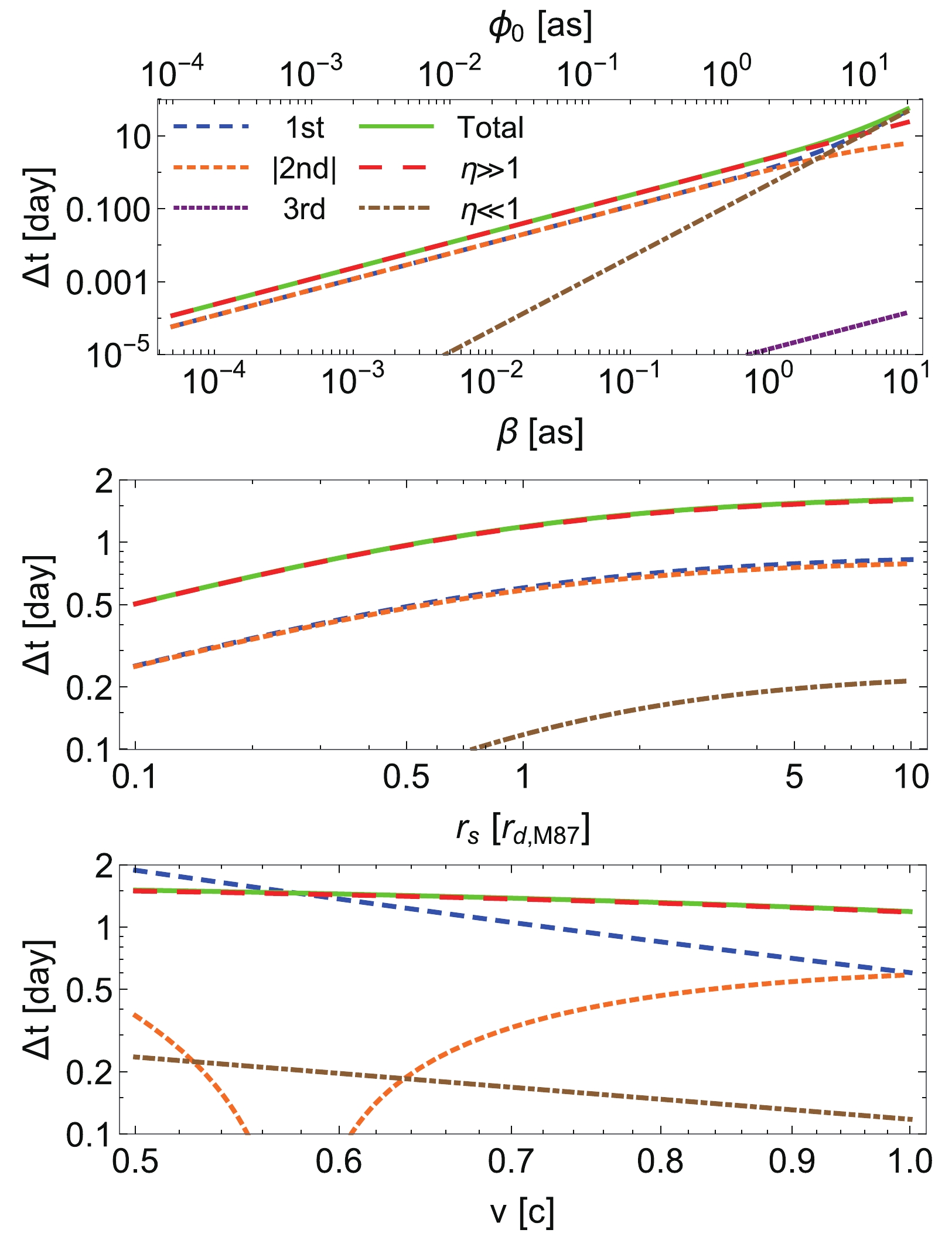

Figure 2.  (color online) Time delay caused by the M87 supermassive BH as a function of $\beta$ (or $\phi_0$) (top), $r_s$ (middle), and v (bottom). The parameters selected are $r_s = r_d$, $\phi_0 = 1$ [as] and $v = c$, except for the parameter that is varied in the x-axis of each subplot. The 1st, |2nd|, 3rd, and "total'' curves correspond to the first, absolute value of the second, third, and all three terms of Eq. (34), respectively. The $\eta\gg 1$ and $\eta\ll 1$ curves correspond to Eqs. (36) and (37).

The first subplot indicates that as $\beta$ increases, the first and second terms of Eq. (34) (or (38)) have similar values until approximately $\beta\approx 2$ [as], beyond which the first term dominates the second one. Moreover, the first two terms are significantly larger than the third one in the entire range. When $\beta \lesssim 4$ [as] and $\beta \gtrsim 4$ [as], the total time delay approaches the $\eta\gg 1$ and $\eta \ll 1$ limits, respectively. In the second subplot, in the entire range of $r_s$, the first and second terms of Eq. (34) (or (38)) are comparable, and their combination becomes the total time delay, which is approximated by the $\eta\gg 1$ limit. In the last subplot, as v varies from $0.5c$ to c, the value of the first term decreases to that of the second term, which increases from negative to positive. Again, their combination forms the total time delay, which is approximated by the $\eta\gg 1$ limit. We can verify that, for these parameters or parameter ranges, all the behaviors described above perfectly match the predictions of Eqs. (34)- (39).

Since both the supernovas and GW+GRB events emit two types of relativistic signals (almost) simultaneously, some researchers have proposed using the difference between the time delays of both types of signals to constrain their properties [25, 28]. Using Eq. (38) for signals with velocities $v_1$ and $v_2$, the time delay difference becomes

where $\Delta v = v_1-v_2$. Similar to Eq. (38), when $\eta\ll 1$, both terms in the square bracket of Eq. (40) are at the same order. Otherwise, the first term dominates. For spacetimes with $\gamma = 1$, the second term vanishes and this reduces to Eq. (38) of Ref. [28]. Equation (40) suggests that for all SSS spacetimes, the time delay difference also relies on only two parameters M and $\gamma$. In all spacetimes where $\gamma = 1$, this time delay difference becomes completely equivalent to that of the Schwarzschild spacetime with the same mass. The corresponding analysis for neutrinos and GW/GRB time delay was conducted in Ref. [28]; therefore, it is not repeated here.

We have developed a perturbative method to compute the total travel time in any SSS spacetime for signals with general velocities. The result, Eq. (26), takes a quasi-series form of $1/b$. Only the first two orders of this result contribute to the leading order(s) of the time delay $\Delta t$, expressed in Eq. (38), between different images of GL. $\Delta t$ depends on the mass M and PPN parameter $\gamma$ of the metric functions. This result reveals that in the weak field limit, high order parameters in asymptotic expansions of the metric functions, such as effective charges, have a significantly smaller effect on $\Delta t$ than M and $\gamma$. The difference of the time delays for different types of signals is also demonstrated to take a universal form to the leading order(s), still determined by M and $\gamma$.

It would be interesting to observe whether this method can be generalized to other types of spacetimes for parameters other than M and $\gamma$ to have a considerable effect on the time delays and their difference. Such spacetimes include at least stationary axisymmetric spacetimes, asymptotically non-flat spacetimes, and non-static/stationary spacetimes [39]. We are currently researching these.

We thank Dr. Nan Yang and Mr. Ke Huang for valuable discussions.

The $y \left( \dfrac{u}{b} \right)$ defined in Eq. (18) can be dismantled into five factors:

In order to expand them into series of $u/b$, the second, third, and fifth factors are ready, and we must focus on the first and fourth factors, $f_1$ and $f_4$

For $f_4$, note that $q = q(u/b)$ and $q(x)$ is defined as the inverse function of $p(x)$, which is given in Eq. (10). Clearly, if the series expansion of $p(x)$ and $q(u/b)$ at small $u/b$ are known, the series of $f_4$ can be obtained. However, the series of $p(x)$ can be simply obtained from its definition (10) when the metric expansions (20) are known. Explicitly, substituting Eq. (20) into (10) (and with the aid of a computer symbolic system to simplify the tedious algebra), we obtain, to the first three orders,

Using the Lagrange inversion theorem in Calculus, its inverse series can be obtained as

Obtaining the derivative of $p(x)$ in Eq. (A4) and then substituting Eq. (A5) into it, the series of the $p^\prime (q)$ factor in $f_4$ can be computed. Using this, as well as Eq. (A5), the series form of the entire $f_4$ can be known in terms of the metric expansion coefficients.

When the series (A5) of $q(u/b)$ is known, compositing it with the metric expansions (20) and substituting them into Eq. (A2), the series of $f_1$ can also be known. Grouping the series of $f_1$ and $f_4$with the second, third, and last factors of $y(u/b)$, we obtain the series of the form (19) with coefficients (21).

A few comments are necessary here. First, the key step in these computation is the inversion from $p(x)$ in Eq. (A4) to $q(x)$ in (A5). This is not used frequently in common scientific and engineering applications of series expansion. However, it is not a difficult step and can be performed relatively easily using the Lagrange inversion theorem. Second, although the remainder of the computations are conceptually simple series multiplications or compositions, computation by hand can be tedious; therefore, a computer symbolic system was used. Third, because of this, a significantly higher order of the the expansion coefficients $y_n\; (n\geqslant 3)$ can also be obtained depending on the complexity of the metric expansions (20). For example, for simple spacetime such as the Schwarzschild metric, $y_n$ up to $n = 12$ can be obtained using a personal computer within a reasonable time.