Off-equatorial deflections and gravitational lensing in Kerr spacetime and the effect of spin

The deflection and gravitational lensing (GL) of light rays are fundamental features of signal motion in curved spacetimes. The early confirmation of the former established general relativity as a more accurate description of gravity [1]. GL has become an important tool in astronomy, from measuring the lens mass and mass distribution [2] to studying the properties of dark mass and dark energy [3, 4]. With advancements in observation technologies, particularly the rapid development of black hole (BH) observations (e.g., Event Horizon Telescope, see [5, 6]), the physics of bending and GL of test particles has become essential for the understanding of the relevant observation results.

Theoretically, the deflection and GL of test particles are most easily understood and thoroughly studied in static and spherically symmetric (SSS) spacetimes or in the equatorial plane of stationary and axisymmetric spacetimes. Different techniques, such as the Gauss-Bonnet-theorem-based geometrical method [7−11] and perturbative methods [12−14], have been used to study deflections of not only null signals but also maissive particles. Various effects, such as the finite distance effect of the source and detectors [15−17], effects of the spacetime parameters (spin, charges [18], magnetic field [19] etc.), and properties of test particles (spin [20] and charge [21, 22]), have been extensively investigated in recent years. However, observationally, the Kerr BH is still one of the most simple and natural BH candidates considered by astronomers [5, 7].

The deflection of test particles and GL of light rays in Kerr spacetime have also been intensively studied. Although relevant numerical packages can often yield the general motions in this spacetime [23], analytical works on deflection and GL focus on the motion in the (quasi-)equatorial plane [12, 24−30]. The following are examples of analytical works on non-equatorial plane motions in the Kerr spacetime. Wilkins investigated the frequencies of the bound orbit in both the $\theta$ and $\phi$ directions [31]. Fujita and Hikida studied the bound timelike orbit solution in terms of Mino time [32]. Hackmann and Xu classified motions of test particles in Kerr and KN spacetimes [33, 34]. Among works most relevant to this paper, Bray calculated the deflection angles of null rays in Kerr spacetime in terms of the conserved constant of the motion [35]. Sereno and De Luca updated this research and solved the image positions using some approximate geometrical relations [36]. Kraniotis determined image locations for observers with certain particular latitudes [37]. Gralla and Lupsasca discussed the highly bent rays and properties of photon rings in Kerr BH spacetime [38].

However, the abovementioned works did not systematically consider the finite distance effect of the source and observer. The lens equations used were also based on the first-order approximation of the geometrical relations linking the angle of the source against the lens-detector axis and the apparent angle. In this paper, we develop a perturbative method that can compute the deflection and GL of test particles with arbitrary orientation directions in the Kerr spacetime. Moreover, the method can consider the finite distance effect of the source and observer, which enables the use of the exact GL equations to obtain the image positions and their magnifications as well as time delays. Furthermore, we do not limit the trajectories to light rays but consider test particles with general asymptotic velocity, i.e., massive particles are also included. The deflection and GL of massive particles have attracted more interest in recent years [9−11, 13, 14, 16, 18, 39] owing to the rapid development of neutrino [40−42] and cosmic ray (see [43] and references therein) observation technologies, the discovery of gravitational waves, and the massiveness of gravitational waves in some beyond general relativity theories [44, 45].

In this work, we show that the deflection angles in Kerr spacetime with mass $M$ in the weak deflection limit (WDL) in both the $\phi$ and $\theta$ directions can be expressed in quasi-power series forms of $M/r_0$ and $r_0/r_{\mathrm{s,d}}$ , where $r_0,\,r_{\mathrm{s,d}}$ are the minimal radial coordinate of the trajectory and the source and detector radial coordinates, respectively. The coefficients of these series are functions of $\hat{a}$ , the spin angular momentum per unit mass, and $v$ (or $E$ ), the asymptotic velocity of the test particles. After solving a set of exact GL equations, we will determine the image positions and magnifications of a source located at arbitrary azimuthal and zenith angles using these deflections. The dependence of these quantities and the time delay between images on the spacetime spin size and its orientation and other parameters will be shown explicitly. We also use these results to discuss some potential applications in astronomical observations.

The remainder of this paper is organized as follows. In Sec. II, we introduce the basic setup of the problem. In Sec. III, the perturbative method is developed and used to express the deflections as power series. The GL equations are solved in Sec. IV to obtain the image locations, magnifications, and time delays. The effects of various parameters on them are also investigated. Sec. VI discusses a few potential applications of the results and concludes the paper. Throughout the work, we use the natural units $G=c=1$ .

The Kerr spacetime with Boyer-Lindquist coordinates $(t,r,\theta,\phi)$ can be described by the following metric:

where

and $a=J/M$ is the angular momentum per unit mass of the BH, with $M$ being its total mass. The motion of test particles in this spacetime is governed by the geodesic equation

where $\sigma$ is the proper time of massive particles or affine parameter of null signals. Using the metric (1), after the first integrals, this becomes [46]

where

and $m,\,E,\,L,\,K$ are the mass, conserved energy and angular momentum of the test particle, and Carter constant, respectively. In asymptotically Minkowski spacetimes, including the Kerr one, $E$ can be related to asymptotic velocity $v$ (the spatial components of the four-velocity) of the massive particle observed by a static observer far from the center, using the relation

For the null signal, $m$ approaches zero but $v$ approaches 1, and $E$ is still finite. For the equations and results throughout this paper, we can always obtain the null limit by taking $v\to 1$ . One of the main motivations for this work is to obtain the deflection of the test particles that are not restricted to the equatorial plane. Hence, using Eqs. (5a) and (5b), we first obtain

Here, $s_\theta$ and $s_r$ are two signs introduced when taking the square root in Eqs. (5a) and (5b), respectively. Using Eqs. (5a) and (9) in the first and last terms, respectively, on the right-hand side of Eq. (5c), we obtain

When proper initial conditions are given, integrating Eqs. (9) and (10) from the source to detector will yield the deflection in the $\phi$ and $\theta$ directions, respectively. If we let $r_ \mathrm{s}$ (or $r_ \mathrm{d}$ ) vary, then knowing the integral results of Eqs. (9) and (10) is equivalent to knowing solutions $\phi(r)$ and $\theta(r)$ .

Before conducting more detailed computations, we provide a few comments regarding these equations and their integrals. First, note that according to Ref. [33], a few types of motion exist in the Kerr spacetime when the particle is not limited to the equatorial plane. The type we will study is classified as the IVb case, which is a flyby orbit. In other words, the particle will travel from a large distance to reach a periapsis and then return to another large distance. In this case, we can adjust the orbit parameters such that the periapsis is far from the event horizon; therefore, the deflection of the test particle is generally weak, which is essential for the feasibility of the weak field perturbative study. In this limit, we can safely assume that the $\theta$ coordinate will experience only one local extremum along the entire trajectory. We denote this extreme value as $\theta_ \mathrm{e}$ . If the signal flies by the lens from above (or below) the equatorial plane, $\theta_ \mathrm{e}$ will be a minimum (or maximum), whereas $\cos\theta_ \mathrm{e}$ will be a local maximum (or minimum).

With the above consideration, we can integrate Eqs. (9) and (10) from the source located at $(r_ \mathrm{s},\,\theta_ \mathrm{s},\,\phi_ \mathrm{s})$ to the detector at $(r_ \mathrm{d},\,\theta_ \mathrm{d},\,\phi_ \mathrm{d})$ to obtain the following relation:

Here, $r_0$ is the minimum radial coordinate along the trajectory, and $\theta_ \mathrm{e}$ is the extreme value of the $\theta$ coordinate. $s_{r\theta}=\pm1$ and $s_l=\pm1$ are the signs induced from Eqs. (9) and (10) when performing the integrals. Here, $s_l$ is the same as the sign of the orbital angular momentum introduced in Eq. (15). $r_0$ and $\theta_ \mathrm{e}$ can be related to conserved constants $L,\,K$ , and $E$ through their definitions

From Eqs. (5a) and (5b), we observe that the above equation is equivalent to determining the roots of the right-hand sides of Eqs. (6) and (7) by setting them equal to zero. Using these, we obtain the analytical expression for $\theta_ \mathrm{e}$ in terms of $L,\,K$ , and $E$

$r_0$ is a root of and order four polynomial and is too lengthy to show here. Note that $L$ and $K$ can be expressed in terms of $r_0,\,\theta_ \mathrm{e}$ , and $E$

where

and $s_l$ in front of $\chi$ is valid in the WDL. These relations can be used to replace $L$ and $K$ in integrals in Eqs. (11) and (12) later.

Among the six coordinates, $(r_ \mathrm{s},\theta_ \mathrm{s},\phi_ \mathrm{s})$ and $(r_ \mathrm{d},\theta_ \mathrm{d},\phi_ \mathrm{d})$ , we assume that $r_ \mathrm{s},\,r_ \mathrm{d}$ , and $\theta_ \mathrm{s}$ are known. $\phi_ \mathrm{s}$ and $\phi_ \mathrm{d}$ are unnecessary to know a priori, and indeed $\Delta\phi\equiv\phi_ \mathrm{d}-\phi_ \mathrm{s}$ is the deflection angle we desire to solve. We also note that the integral in Eq. (12) is exactly deflection $\Delta \phi$ in the $\phi$ direction. For deflection $\Delta\theta\equiv \theta_ \mathrm{d}+\theta_ \mathrm{s}-\pi$ in the $\theta$ direction, we observe from Eq. (11) that when $r_ \mathrm{s},\,r_ \mathrm{d}$ , and $\theta_ \mathrm{s}$ are given, and if we can perform the integral in this equation, then solving the resultant algebraic equation will enable us to determine $\theta_ \mathrm{d}$ and consequently $\Delta\theta$ .

One of the main efforts of this work is to determine proper tractable methods to perform these integrals. We show in the next section that a perturbative method exists to systematically approximate these deflections, and the result takes a dual series form of $M/r_0$ and $r_0/r_{\mathrm{s,d}}$ .

The key to successfully performing integrals (11) and (12) is to determine a proper method to expand the integrands into integrable series, which enables approximations to any desired accuracy. The WDL provides a natural expansion parameter, ratio $M/r_0$ . Before conducting this expansion, we must mention that the orbital angular momentum $L$ and Carter constant $K$ of the test particle are not easily measurable. Therefore, we must replace them in Eqs. (11) and (12) with Eqs. (15) and (16). For simpler notations, introducing the new integration variables,

as well as the auxiliary notations

and then performing the expansions using $M/r_0$ as a small parameter, Eqs. (11) and (12) become

where $f_{r,i},\,f_{\theta,i},\,g_{r,i},\,g_{\theta,i}$ are the Taylor expansion coefficients of the integrands whose exact forms can be determined easily. Here, we list their first few orders:

where $\hat{a} \equiv a/M$ .

Because all $f_{r,i}$ and $g_{r,i}$ are polynomials of $p$ and $f_{\theta,i}$ and $g_{\theta,i}\; (i>0)$ are polynomials of $c^2$ , the integrability of expansions in Eqs. (19) and (20) relies on the integrability of the following integrals:

Fortunately, they are always integrable (see Appendix A for the proof), and this guarantees that we can obtain a series solution for the deflection angles.

After integration, the results for Eqs. (19) and (20) become

Here, coefficient functions $F_{r,i},\,F_{\theta,i},\,G_{r,i},\,G_{\theta,i}$ are integration results of terms containing $f_{r,i},\,f_{\theta,i},\,g_{r,i},\,g_{\theta,i}$ , respectively, and therefore are also functions of the corresponding integration limits. The first few of them, for $j=\{\mathrm{s},\,\mathrm{d}\}$ , are

We must be careful when interpreting Eqs. (24) and (25). Although Eq. (25) appears as a series of $(M/r_0)$ with $G_{r,i}$ and $G_{\theta,i}$ as the coefficients of deflection $\Delta\phi$ , it is still not the true final perturbative series of $(M/r_0)$ as in the case in the equatorial plane. The first reason is that $p_\mathrm{s,d}$ has a dependence on $r_0$ (see Eq. (18)). The second and stronger reason is that, as indicated in the last section, among parameters $r_{\mathrm{s,d}},\,\theta_\mathrm{s,d},\,r_0$ , and $\theta_ \mathrm{e}$ , not all of them are independent. $\theta_ \mathrm{d}$ can be fixed using other parameters including $r_0$ , and this must be considered when attempting to obtain an $(M/r_0)$ series of $\Delta\phi$ . This relation can be derived from Eq. (24) using two methods, the perturbative and Jacobi elliptic function methods, respectively. Here, we directly present the result of this relation but postpone its derivation to Appendix B.

where

and

To compute deflection angle $\Delta\phi$ , we need only substitute Eq. (27) into (25) and recollect terms involving $G_{\theta,i}$ into a power series in $(M/r_0)$ with new coefficients $G_{\theta,i}^\prime$ . Thereafter, $\Delta\phi$ finally becomes

where $G_{r,i}$ is still given by Eq. (26e), and the first three orders of $G_{\theta,i}^\prime\; (i=0,1,2)$ are

The null limit of this deflection can be obtained easily by taking $v=1$ , resulting in, to the leading order

We have also verified that $\Delta\phi$ in Eq. (30) has the correct equatorial plane limit. Specifically, if we let $\theta_ \mathrm{s}\to\pi/2, \theta_ \mathrm{e}\to\pi/2$ , this deflection angle will reduce to the result computed purely in the equatorial plane for particles with arbitrary asymptotic velocity [17].

To observe the finite distance effect more clearly, we can expand $\Delta\phi$ in Eq. (30) in the small $p_\mathrm{s,d}$ limit:

where $\varepsilon$ indicates the infinitesimal of either $(M/r_0)$ or $p_\mathrm{s,d}$ , and the coefficients are

where recalling $t_ \mathrm{s}=\tan\theta_ \mathrm{s},\; s_i=\sin\theta_i\; (i=\mathrm{s,d})$ and we have set, here and for later use,

Note that the higher order coefficients in Eq. (33) can also be determined easily but are too tedious to show here. If we take the infinite distance limit, then this becomes

If we further take the null limit of $v=1$ , this simplifies to

For the deflection in the $\theta$ direction, Eq. (27) provides the desired solution for $\theta_ \mathrm{d}$ when $r_{\mathrm{s,d}},\,\theta_\mathrm{s,e}$ , and $r_0$ are known. In other words, deflection $\Delta\theta$ becomes

where $c_ \mathrm{d}$ is given by Eq. (27). For null rays, this deflection becomes, to the leading order

To have a better understanding of this result, similar to the case of $\Delta\phi$ , we can also expand it for small $p_\mathrm{s,d}$ and find

where the coefficients are

Setting $p_\mathrm{s,d}$ to zero, this yields the deflection in the $\theta$ direction for source and detector at infinite radii:

Further setting $v=1$ , the null limits of this deflection becomes

When studying GL due to the lens, Eqs. (27) and (30) enable us to solve for $(\theta_ \mathrm{e},\,r_0)$ when source location $(r_ \mathrm{s},\,\theta_ \mathrm{s},\,\Delta\phi)$ and detector location $(r_ \mathrm{d},\,\theta_ \mathrm{d},\,0)$ are fixed. Here, without loss of generality, we can set the $\phi$ coordinate of the detector to zero, which means that the source $\phi$ coordinate will be $\Delta\phi$ . Solutions $(r_0,\,\theta_ \mathrm{e})$ can then be directly used in the apparent angle formula Eq. (46) to yield the apparent angles of the images.

In this section, we demonstrate how considering the series solution of the deflection angles with finite distance effect can aid us in solving $r_0$ and $\theta_ \mathrm{e}$ naturally and more precisely. These quantities provide the desired apparent angles and their magnifications of the GL images using a set of exact formulas in Sec. IV.B.

With the deflection in both $\theta$ and $\phi$ directions known, we can attempt to solve for the apparent angles of the lensed images using the GL equations. Such GL equations are often formulated using approximate geometrical relations that link the source and detector locations, the intermediate variables such as $r_0$ and $\theta_ \mathrm{e}$ , deflection angles $\Delta\phi,\,\Delta\theta$ , as well as the desired apparent angle(s), which has two components $(\alpha,\,\beta)$ in our case. In Fig. 1, we adopt the common setup of the detector's local inertial frame, whose basis axes consist of detector-lens direction $\hat{r}_ \mathrm{d}$ , and directions $\hat{\theta}_ \mathrm{d}$ and $\hat{\phi}_ \mathrm{d}$ parallel to the $\hat{\theta}$ and $\hat{\phi}$ bases, respectively, of the spacetime coordinates.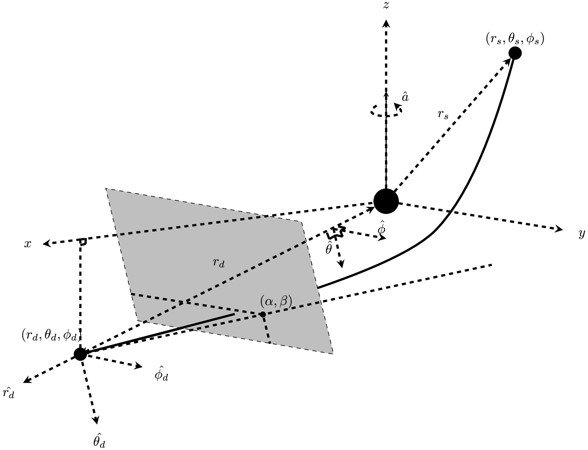

Figure 1.  Schematic of the deflection and lensing in the WDL in Kerr BH spacetime. The source and detectors are located at $(r_ \mathrm{s},\theta_ \mathrm{s},\phi_ \mathrm{s})$ and $(r_ \mathrm{d},\theta_ \mathrm{d},\phi_ \mathrm{d})$ , respectively. The gray box represents a patch of the celestial plane of the detector. The apparent angles of the images on this plane are also indicated. $(\alpha,\,\beta)$ are the small apparent angles of the image against the projected axis of $+\hat{z}$ and $+\hat{y}$

In this work, our set of the GL equation consists of two equations. The first set is simply the definitions of the deflections in the $\phi$ and $\theta$ directions:

where $\Delta\phi$ and $\Delta\theta$ are expressed as in Eqs. (30) and (38), and $\delta\phi$ and $\delta\theta$ are two small deviation angles characterizing the location of the source relative to the lensing-observer axis when the lens is not present. We argue that this set of GL equations is more exact because unlike many others, they are simply definitions of the deflection, and their establishment requires no other geometrical approximations. Using this set of equations, when quantities $a,\,M$ and $(r_ \mathrm{s},\,\theta_ \mathrm{s},\,\phi_ \mathrm{s}),\,(r_ \mathrm{d},\,\theta_ \mathrm{d},\,\phi_ \mathrm{d}=2\pi)$ are given in advance, we can solve for the intermediate variables, i.e., minimal radial coordinate $r_0$ and extreme angle $\theta_ \mathrm{e}$ that enable the test particle to reach the detector. These two quantities can also be interchanged with the other pair of kinetic variables $(L,\,E)$ of the test particle. Note that without loss of generality, we have fixed $\phi_ \mathrm{d}=2\pi$ , and in the WDL, $\phi_ \mathrm{d}-\phi_ \mathrm{s}$ is typicllat very close to $\pi$ .

In practice, because Eqs. (30) and (38) have a more complicated dependence on $r_0$ and $\theta_ \mathrm{e}$ , when substituting into Eq. (44), we will use their expanded forms, i.e., Eqs. (33) and (40) with terms of combined order higher than two truncated. Inspecting these two equations carefully, we can observe that their dependence on $r_0$ can be converted to a polynomial form. From Eqs. (34g) and (41g), we observe that the second order in the expansion of $(M/r_0)$ is also the minimal order that the effect of spacetime spin $\hat{a}$ will appear. Therefore, any attempt to study the off-equatorial plane deflection and lensing should retain the deflection angles to at least this order, which is also our approach in this work. Otherwise, the off-equatorial motion will simply be a simple rotation of the equatorial motion in Schwarzschild spacetime because spin $\hat{a}$ is not considered. However, for the dependence of this set of equations on $\theta_ \mathrm{e}$ , we observe that these two equations are both linear combinations of $\sin(n x_ \mathrm{s})$ and $\cos(n x_ \mathrm{s}) (n=0,\,1,\,2)$ , which can also be converted to polynomials of $\tan(x/2)$ . However, to the order we are interested in, these polynomials do not allow simple analytical forms for their solutions. More precisely, to include the effect of $\hat{a}$ , we find that $\tan(x/2)$ should be a root of an order tenth-order polynomial. However, when $\tan(x/2)$ is obtained, $r_0$ can be simply evaluated (not solved) from a polynomial involving $\tan(x/2)$ . Therefore, in the following, we use the numerical methods to solve $r_0$ and $\tan(x/2)$ .

In addition to these two equations, we provide a selection condition of the solutions related to the initial conditions. When $s_{r\theta}>0$ (or equivalently $s_\theta>0$ because we always use $s_r>0$ ), Eq. (9) implies that the trajectory initially moves toward decreasing $\theta$ ; therefore, we will require that $\theta_e$ be smaller than $\theta_ \mathrm{s}$ . In contrast, if $s_{r\theta}<0$ , we will require that $\theta_ \mathrm{e}>\theta_ \mathrm{s}$ .

In Figs. 2−5, we plot the solved $r_0$ and $\theta_ \mathrm{e}$ as functions of variables $\delta\phi,\,\delta\theta,\,\theta_ \mathrm{s},\,\hat{a}$ , and $r_{\mathrm{s,d}}$ using Sgr A* as the central lens. We utilize its data $M=4.1\times 10^6M_\odot$ and $r_ \mathrm{d}=8.34$ kpc [6]. In principle, if we let the spacetime spin to be negative and the locations of the source and detector to be switched, then we can restrict the non-equivalent parameter space to $\delta\phi>0,\,\delta\theta>0,\,\theta_ \mathrm{s}\in [0,\pi/2]$ . However, to show the lensed images more comprehensively, in some of the plots in the following, we will consider negative $\delta\theta,\,\delta\phi$ . The choice of other parameters is provided in the caption of each plot.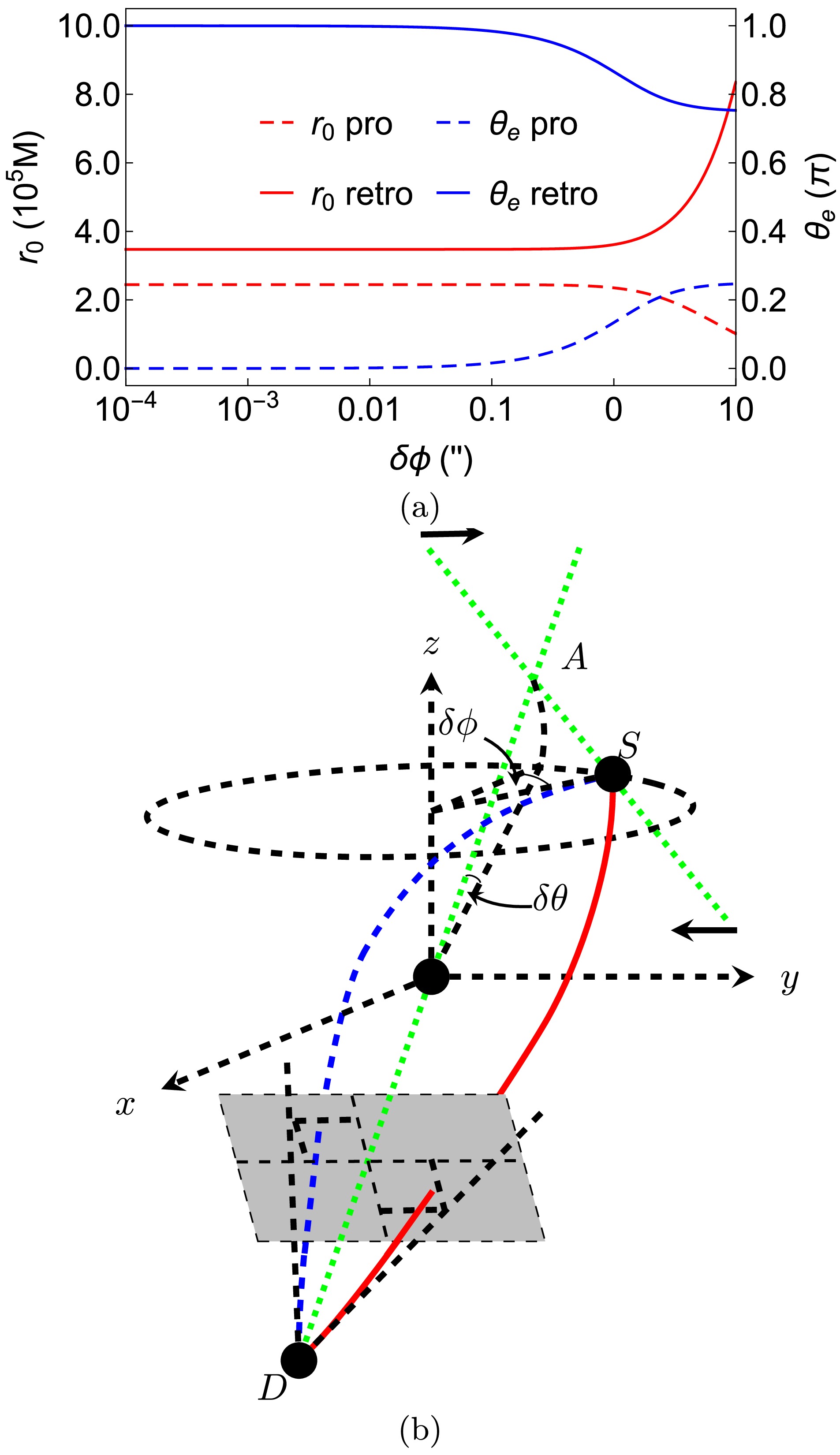

Figure 2.  (color online) (a) Dependence of $r_0$ and $\theta_ \mathrm{e}$ on $\delta\phi$ . We fix $\theta_ \mathrm{s}=\pi/4,\,\delta\theta=1^{\prime\prime},\,\hat{a}=1/2,\,r_ \mathrm{s}=r_ \mathrm{d},\,v=1$ in this plot. (b) Decrease in $\delta\phi$ .

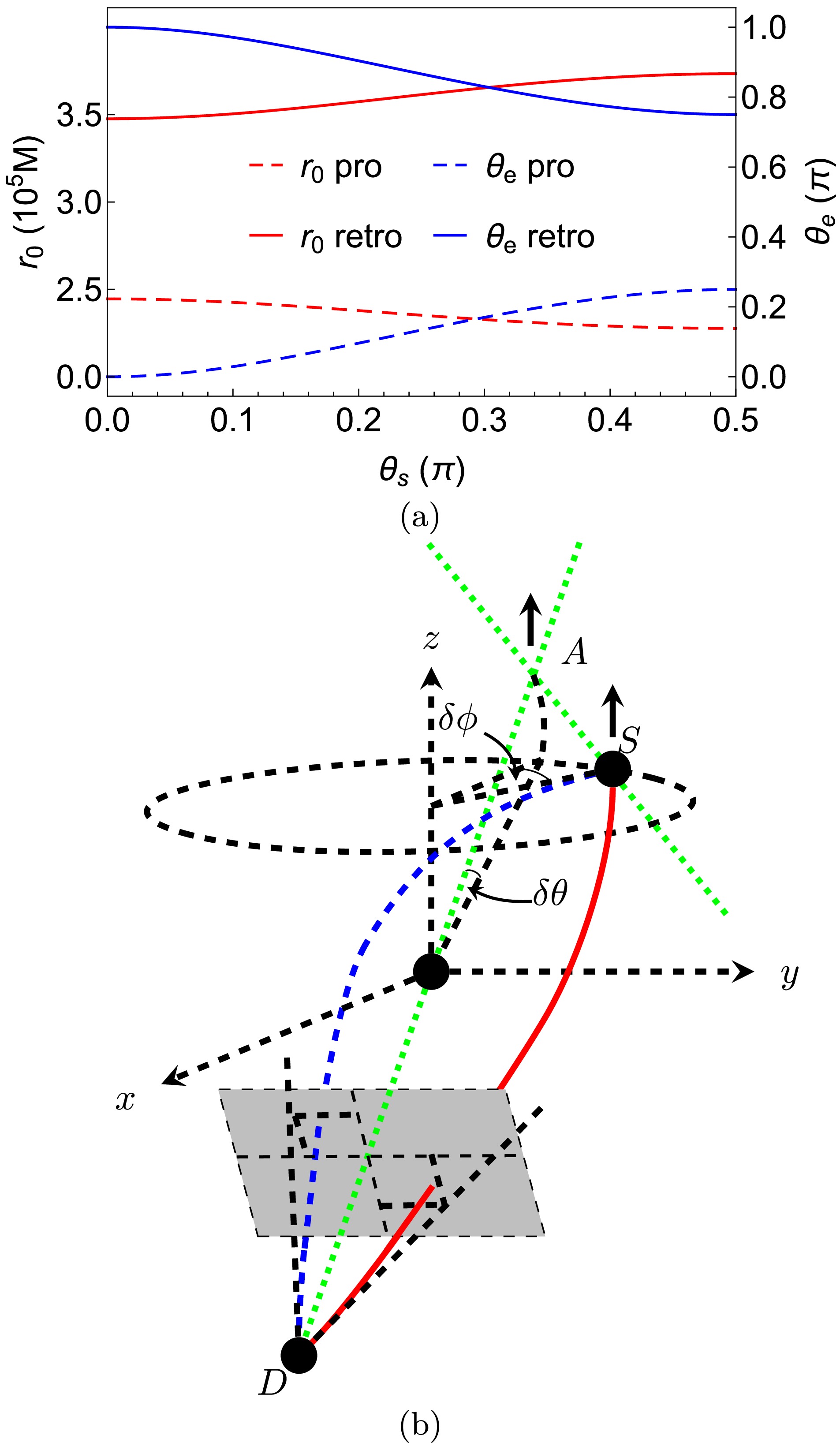
Figure 3.  (color online) (a) Dependence of $r_0$ and $\theta_ \mathrm{e}$ on $\theta_ \mathrm{s}$ . We fix $\delta\phi=1^{\prime\prime},\; \delta\theta=1^{\prime\prime},\,\hat{a}=1/2,\,r_ \mathrm{s}=r_ \mathrm{d},\,v=1$ in this plot. (b) Change in the trajectories as $\theta_\mathrm{s}$ decreases while keeping $\delta\theta$ an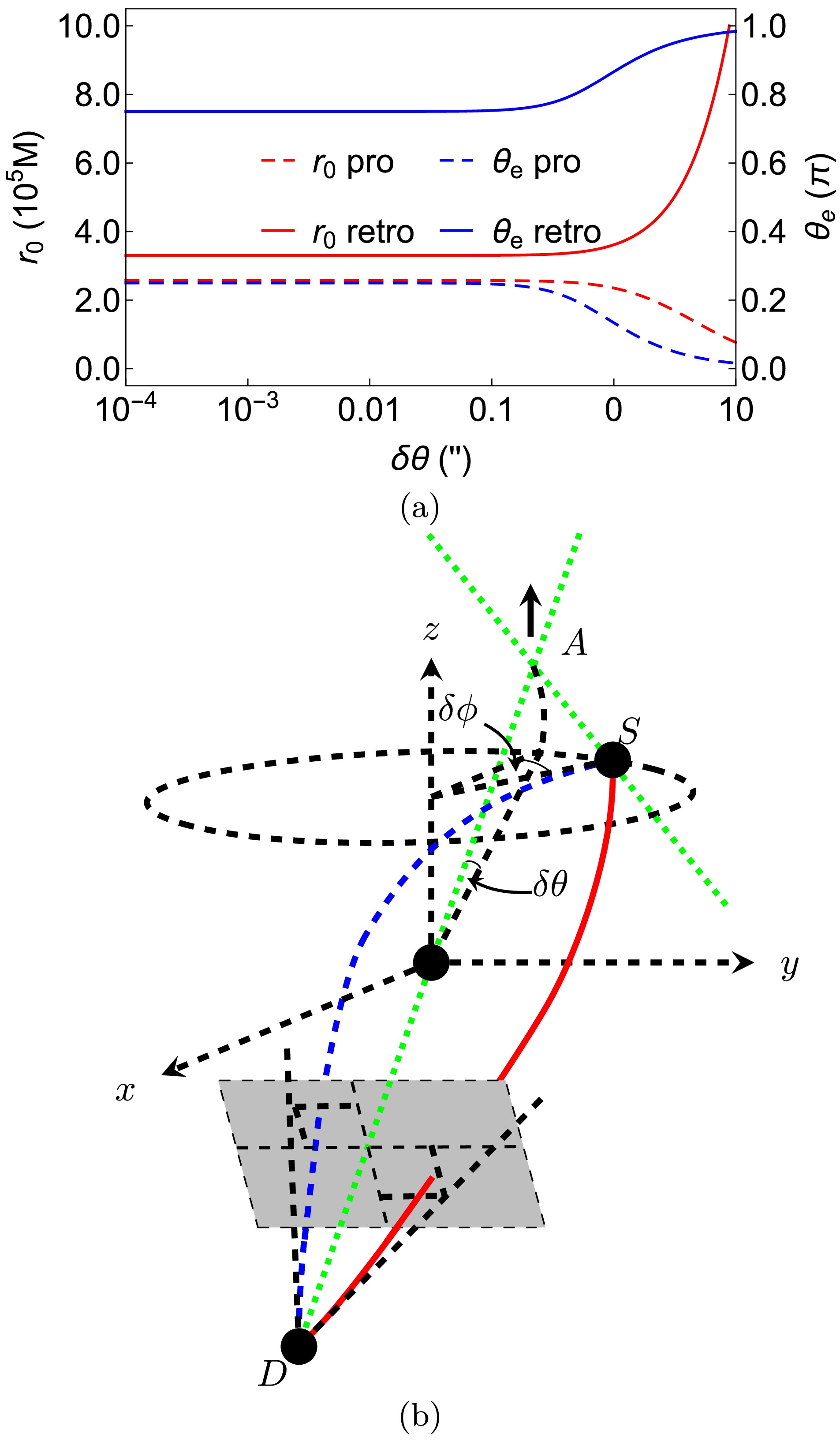d $\delta\phi$ fixed.

Figure 4.  (color online) (a) Dependence of $r_0$ and $\theta_ \mathrm{e}$ on $\delta\theta$ . We fix $\delta\phi=1^{\prime\prime},\,\theta_ \mathrm{s}=\pi/4,\,\hat{a}=1/2,\,r_ \mathrm{s}=r_ \mathrm{d},\,v=1$ in this plot. (b) Variation in $\delta\theta$ .

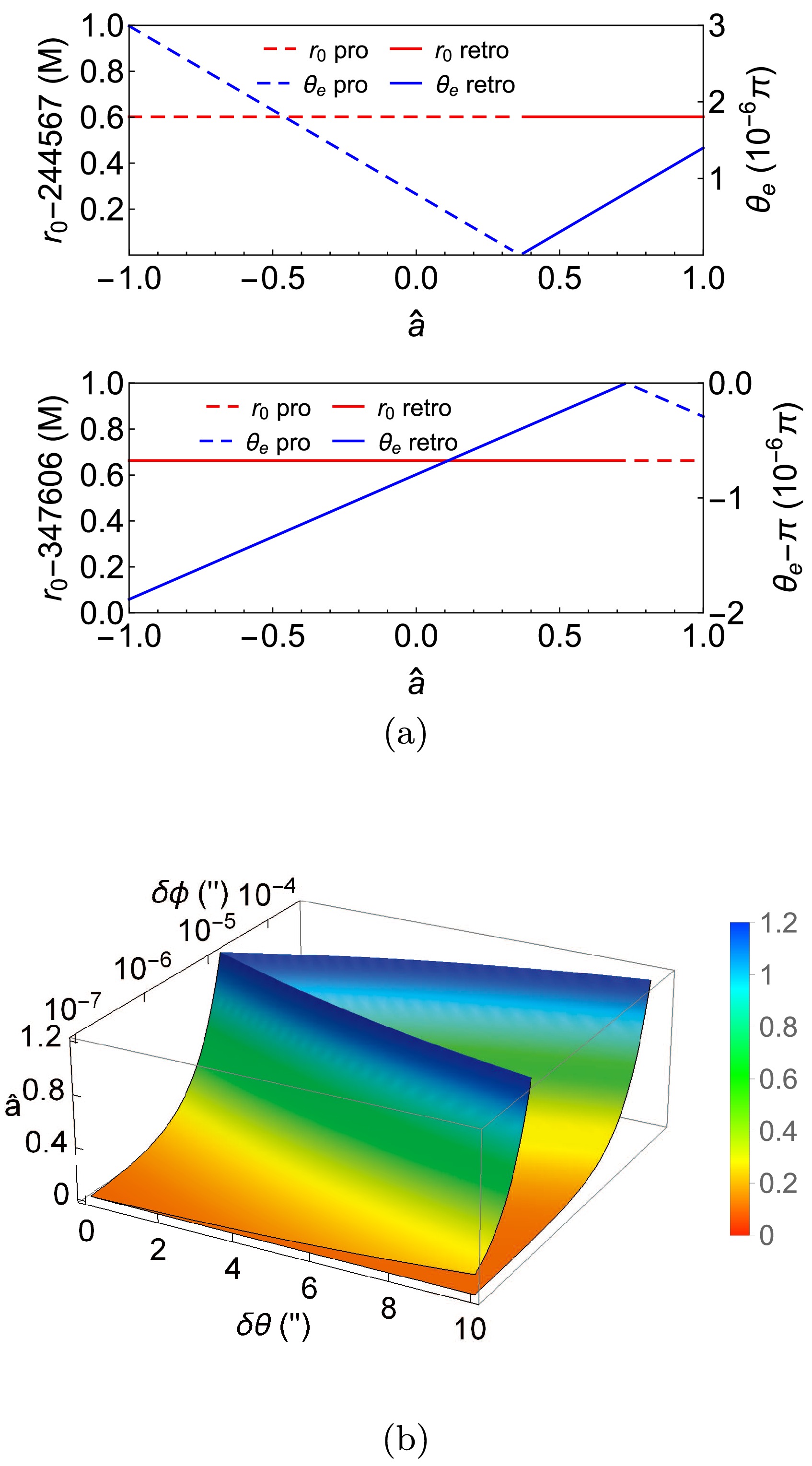
Figure 5.  (color online) (a) Dependence of $r_0$ and $\theta_{ \mathrm{e}\pm}$ on $\hat{a}$ . We fix $\delta\theta=1^{\prime\prime}, \delta\phi=5*10^{-6\prime\prime}, \theta_ \mathrm{s}=\pi/4,\,r_ \mathrm{s}=r_ \mathrm{d},\,v=1$ . (b) The critical $\hat{a}_{c\pm}$ . We fix $\theta_ \mathrm{s}=\pi/4,\,r_ \mathrm{s}=r_ \mathrm{d},\,v=1$ in this plot.

Let us indicate a few features of the solution process and results. First, we observe that for each set of parameters and among the four different possible combinations of signs $s_{r\theta}$ and $s_l$ , only two combinations allow physical solutions to $r_0$ and $\theta_ \mathrm{e}$ . In most of the parameter space, one of these allowed trajectories will be prograde with respect to the $+z$ axis, whereas the other will be retrograde. In this paper, by prograde and retrograde, we specifically mean that the trajectories rotate anticlockwise and clockwise around the $+\hat{z}$ directions, respectively. No retrolensing is involved because we discuss only the weak deflection cases in this work. We denote the minimal radii and extreme $\theta$ coordinate of the prograde trajectory as $(r_{0+},\,\theta_{ \mathrm{e}+})$ and those of the retrograde trajectory as $(r_{0-},\,\theta_{ \mathrm{e}-})$ . Because $\theta_ \mathrm{s}\leq \pi/2$ , when $\theta_ \mathrm{e}$ is a minimum (or maximum), the trajectory reaches the detector from above (or below) the equatorial plane after bending, as indicated in Fig. 1 by the two solid trajectories.

Second, we would like to indicate two fundamental properties of the trajectories that will aid in the understanding of the results presented in many of the following figures. The first is that when $\delta\phi$ is relatively large (greater than $10^{-4\prime\prime}$ ) for the numerical values of other parameters we have used, the spacetime spin's effect is only secondary compared with that of $\delta\phi$ . This can be understood from Eqs. (44a) and (30) that $\hat{a}$ appears one order higher than $\delta\phi$ or from the deflection angle that $\hat{a}$ appears one order higher than $M/r_0$ . Under these parameter settings, the effect of the spin can be ignored and the physics should be similar to the SSS case, in which the total deflection angle can be approximated as

Subsequently, from our experience with SSS spacetime, we know that when $\delta\phi>0$ , the minimal radial coordinate $r_{0+}$ will decrease, whereas $r_{0-}$ will increase as $\delta\eta$ increases, as in Schwarzschild spacetime [47], regardless of whether the increase in $\delta\eta$ is caused by the increase in $\delta\phi,\,\theta_ \mathrm{s}$ , or $\delta\theta$ . When the effect of $\hat{a}$ is secondary, the second feature of the trajectories is that both trajectories lie essentially within a single plane that contains the source, lens, and detector. With these two fundamental properties in mind, we can then study and more easily understand the effect of various quantities on the extreme $\theta_{ \mathrm{e}\pm}$ by simply drawing this plane in the Cartesian coordinates.

Effect of various parameters

Figure 2 shows the dependence of $r_{0\pm}$ and $\theta_{\mathrm e\pm}$ on $\delta\phi$ . This relationship is one of the main focuses of the GL in SSS or equatorial plane of stationary and axisymmetric spacetimes. As described earlier, each set of fixed parameters has only two physical trajectories, which we denote as $(r_{0+},\,\theta_{ \mathrm{e}+})$ for the prograde one and $(r_{0-},\,\theta_{ \mathrm{e}-})$ for the retrograde one. For the minimal radii, Fig. 2(a) (left axis) shows that, if deflection $\delta\phi$ is larger than the deflection in the $\theta$ direction ( $\delta\theta=1^{\prime\prime}$ ), its effect on the bending of the trajectories would dominate those of the spacetime spin as well as $\delta\theta$ , as can be observed from its contribution to total deflection $\delta\eta$ in Eq. (45). As $\delta\phi$ decreases, $r_{0-}$ would rapidly decrease and $r_{0+}$ would increase, which is a feature qualitatively similar to the case in the equatorial plane [17]. However, as $\delta\phi$ approaches and becomes smaller than $\delta\theta$ , the effect of $\delta\theta$ to the bending will fix the two minimal radii at constant values, as shown by the flat regions in the left part of Fig. 2 (a). For the extreme $\theta_ \mathrm{e}$ of the two trajectories, Fig. 2 (b) (right axis) shows that as $\delta\phi$ decreases, $\theta_{ \mathrm{e}+}$ (or $\theta_{ \mathrm{e}-}$ ) of the prograde (or retrograde) trajectory continues decreasing (or increasing), indicating that the trajectory swings closer to the $z$ axis above (or below) the equatorial plane. As $\delta\phi$ becomes much smaller than $\delta\theta$ , the trajectories primarily bend in the $\theta$ direction, and $\theta_{ \mathrm{e}+}$ and $\theta_{ \mathrm{e}-}$ approach $\pi$ and $0$ indefinitely. We remind the readers that the $\theta$ coordinate along the trajectory does not necessarily deviate weakly from $\theta_\mathrm{s,d}$ even in the WDL, which can be understood in the straight trajectory case in zero gravity. Figure 2 (b) depicts schematically the change of the trajectories as $\delta\phi$ decreases.

Figure 3 shows the effect of $\theta_ \mathrm{s}$ on $r_{0\pm}$ and $\theta_{ \mathrm{e}\pm}$ . Note when adjusting $\theta_ \mathrm{s}$ , we keep $\delta\theta=1^{\prime\prime}=\delta\phi$ a small constant such that $\theta_ \mathrm{d}$ is simultaneously adjusted. First, we observe that, compared with the effect of $\delta\phi$ on these quantities, that of $\theta_ \mathrm{s}$ is much weaker in general: a change in $\theta_ \mathrm{s}$ of about $\pi/2$ causes approximately the same amount of change in $\theta_{ \mathrm{e}\pm}$ and a smaller change in $r_{0\pm}$ than those by a change in $\delta\phi$ of $10^{\prime\prime}$ . However, this is expected both from Eq. (45) and the fact that the approximate alignment of the source-lens-detector is not changed dramatically as $\theta_ \mathrm{s}$ varies. The second feature is that the effects of $\theta_ \mathrm{s}$ on both $r_{0\pm}$ and $\theta_{ \mathrm{e}\pm}$ become stronger as $\theta_ \mathrm{s}$ decreases to zero, i.e., the $z$ axis pole directions, and weaker as it moves toward $\pi/2$ , i.e., the equatorial plane. This is consistent with the first-order terms of Eq. (40), i.e., Eqs. (41b) and (41d), which are proportional to $\cos(x_ \mathrm{s})$ approaching $0$ as $\theta_ \mathrm{s}$ approaches the equatorial plane, and can also be observed by differentiating Eq. (45) with respect to $\theta_ \mathrm{s}$ .

For the effect of $\theta_ \mathrm{s}$ on $r_{0\pm}$ , Fig. 3 (a) (left axis) shows that when the source and detectors are closer to the poles, the minimal radial coordinate $r_{0+}$ (and $r_{0-}$ ) for prograde (and retrograde) motion decreases (and increases) slightly. From our experience [47] with Schwarzschild spacetime with deflection $\delta\eta$ as given in Eq. (45), we can easily anticipate that the two minimal radii should basically assume the shape shown in Fig. 3 (a) as $\theta_ \mathrm{s}$ varies. For $\theta_{ \mathrm{e}\pm}$ , Fig. 3 (a) (right axis) shows that more polar source and detector locations yield more polar $\theta_{ \mathrm{e}\pm}$ . This can be understood from the second property we mentioned above that each trajectory lies basically in one plane containing the source, lens, and detector. We can show by plotting this plane in the Cartesian coordinates that the closer $\theta_ \mathrm{s}$ is to the $+z$ -axis, the closer $\theta_{ \mathrm{e}\pm}$ is to the poles. The change caused by the variation in $\theta_ \mathrm{s}$ is schematically shown in Fig. 3 (b).

The effect of $\delta\theta$ on $r_{0\pm}$ and $\theta_{ \mathrm{e}\pm}$ , as shown in Fig. 4, is related to the effects of $\theta_ \mathrm{s}$ in Fig. 3 and $\delta\phi$ in Fig. 2 through the combination of these three parameters into the total deflection, as in Eq. (45). From Fig. 4 (a) (left axis), we observe that as $\delta\theta$ increases to about $10^{\prime\prime}$ , $r_{0+}$ for the prograde trajectory increases and $r_{0-}$ for the retrograde trajectory decreases. However, the amount of their changes is larger than those in Fig. 2 (a) because of the additional factor of $\sin^2\theta_ \mathrm{s}=1/2$ in Eq. (45). The difference between the effects of $\delta\theta$ and $\delta\phi$ appears in their effects on $\theta_{ \mathrm{e}\pm}$ . An increase in $\delta\theta$ with a fixed $\theta_ \mathrm{s}$ means an increase in $\theta_ \mathrm{d}$ . Therefore, for an increasing $\delta\theta$ but a fixed $\delta\phi$ , we observe that the plane containing the source, lens, detector and the two trajectories will be tilted more vertically towards the $z$ axis. When $\delta\phi>0$ , this effectively increases $\theta_{ \mathrm{e}-}$ and decreases $\theta_{ \mathrm{e}+}$ , as observed in Fig. 4 (a) (right axis). The variation in the trajectories with the increase in $\delta\theta$ is schematically shown in Fig. 4 (b).

Finally, we plot the effect of spacetime spin $\hat{a}$ on $r_{0\pm}$ and $\theta_{ \mathrm{e}\pm}$ in Fig. 5. As mentioned earlier, we observe that when total deflection $\delta\eta$ is larger than a certain value ( $\sim 10^{-5\prime\prime}$ ), the effect of $\hat{a}$ on these quantities is weak such that no noticeable changes are observed in these plots. Therefore, in these figures, we decrease $\delta\phi$ and $\delta\theta$ simultaneously from $10^{-5\prime\prime}$ to about $10^{-7\prime\prime}$ . As the deflections decrease, the influence of $\hat{a}$ begins to appear.

One of the most remarkable characteristics that we observe in Fig. 5 (a) is that when $\delta\phi$ is small, a transition exists between trajectories with different choices of $(s_{r\theta},s_l)$ when $\hat{a}$ passes some critical values. When $\delta\phi$ becomes sub- $\sim 10^{-5\prime\prime}$ , the solution with $(s_{r\theta}=+1,s_l=+1)$ ceases to exist when $\hat{a}$ is larger than $\hat{a}_{c+}$ and that with $(s_{r\theta}=-1,s_l=-1)$ ceases to exist when $\hat{a}$ is larger than another critical value $\hat{a}_{c-}$ . Instead, the above two solutions switch their sign choices to $(s_{r\theta}=+1,s_l=-1)$ and $(s_{r\theta}=-1,s_l=+1)$ , respectively. This means that for $\delta\phi>0,\,\delta\theta>0$ and $\theta_ \mathrm{s}<\pi/2$ , the test particle reaching the detector from bending above (or below) the equatorial plane switches from prograde to retrograde (or vice versa). In other words, the two trajectories intersect with the $z$ axis at $\hat{a}=\hat{a}_{c+}$ and $\hat{a}=\hat{a}_{c-}$ , respectively; therefore, $\theta_{ \mathrm{e}\pm}=0,\,\pi$ as confirmed in Fig. 5 (a).

This observation effectively provides us with the following criterion to solve for $\hat{a}_{c\pm}$ : $\theta_e=0\; \text{or}\; \pi$ . Substituting this into the lensing Eq. (44), we can solve for critical $\hat{a}_{c\pm}$ to the leading order, as a function of $\delta\theta,\,\delta\phi$ and spacetime parameters. In Fig. 5 (b), we plot the exact dependence of $\hat{a}_{c\pm}$ on $\delta\theta$ and $\delta\phi$ while maintaining other parameters such as $\theta_ \mathrm{s},\,r_{\mathrm{s,d}}$ . We observe that the smaller the $\delta\phi$ , the smaller the transition spins $|\hat{a}_{c\pm}|$ , indicating that this switching of the signs is primarily a spacetime spin effect. Moreover, if the spacetime is a BH one ( $|\hat{a}|\leq 1$ ), then only for small $\delta\phi$ does a critical $\hat{a}_{c\pm}$ exist. For $\hat{a}$ below (or above) these two surfaces, the trajectories as shown in Figs. 3−4 with signs $(s_{r\theta}=+1,s_l=+1)$ and $(s_{r\theta}=-1, s_l=-1)$ (or $(s_{r\theta}=+1,s_l=-1)$ and $(s_{r\theta}=-1, s_l=+1)$ ) are the physical solutions, respectively.

A few other characteristics are worth remarking upon for these transitions. First, this plot shows that the transitions depend on $\delta\theta$ much more weakly than on $\delta\phi$ . This is understandable because $\hat{a}$ is along the direction around which the $\phi$ coordinate evolves but not along the direction of the $\theta$ coordinate. This is also consistent with our knowledge about the deflections in the equatorial plane, where the effect of spin $\hat{a}$ is most apparent only when $\delta\phi$ is very small [14]. Second, we also note that when $\delta\phi$ is small and fixed, the spin effect is stronger for a larger $\delta\theta$ in that the corresponding $\hat{a}_c$ is smaller. Third, these transitions can also be considered as caused by the variation in $\delta\theta$ or $\delta\phi$ when other parameters are fixed. In other words, if we fix a constant $\hat{a}$ , then for each $\delta\theta$ , a critical $\delta\phi$ exists, below which the sign choice for $(s_{r\theta},\,s_l)$ would be $(+,-)$ and $(-,+)$ . Finally, some ranges of $\delta\theta$ and $\delta\phi$ exist in which $\hat{a}_{c\pm}$ can exceed the extreme Kerr BH limit of 1. Therefore, for these deflection angles, the transition will not occur if we consider only the BH spacetime case. However, even for the Kerr spacetime with a naked singularity (the $\hat{a}>1$ part in this plot), we emphasize that the critical $\hat{a}_{c\pm}$ still exists and our plot is still valid.

For $r_{0\pm}$ , it was previously known that in the equatorial plane, an increase in $\hat{a}$ will decrease $r_{0+}$ and increase $r_{0-}$ [14]. We observe from the magnified figure that this trend is qualitatively unchanged in the off-equatorial plane case, and it will be more apparent for very small $\delta\theta$ and $\delta\phi$ (e.g., $\sim 10^{-7\prime\prime}$ ). Although the influence of $\hat{a}$ on $\theta_{ \mathrm{e}\pm}$ appears weak, it is more interesting than its effect on $r_{0\pm}$ .

Apparent angles

When $(r_0,\,\theta_ \mathrm{e})$ or $(L,E)$ are solved for a given set of small $\delta\theta$ and $\delta\phi$ , previously, based on some approximate geometrical relations, Refs. [35, 37] developed approximate formulas for the apparent angles of the images observed by a static observer at $(r_ \mathrm{d},\,\theta_ \mathrm{d},\,\phi_ \mathrm{d})$ . However, here, we use the following exact definition of the apparent angles derived from the projection of the test particle trajectory onto the celestrial sphere of the observer (see Fig. 1 for the meaning of these small angles):

Substituting $(\Theta(c_ \mathrm{d}),\,L,\,E)$ into Eqs. (7), (15), (16) and further expanding as series of $M/r_0$ and $r_0/r_ \mathrm{d})$ , they can be transformed to

where we recall that

For the derivation of these formulas, see Appendix C. Note that $r_{0\pm}$ and $\theta_{ \mathrm{e}\pm}$ enter these apparent angles through angular momentum $L$ and Carter constant $K$ , which appears in $\Theta(c_ \mathrm{d})$ . These formulas have the advantage that they are applicable regardless of whether the test particle is bent weakly or strongly, although we focus only on the former case in this work. We have also verified for the weak deflection and equatorial plane limit that $\beta$ approaches $0$ and $\alpha$ yields the corresponding results in Ref. [17] (after switching from impact parameter to $r_0$ ). Moreover, if we are interested in a single apparent angle $\gamma$ between the test particle and the direction of the Kerr BH, this is given by Eq. (C12).

To reveal the dependence of the image positions on parameters $\delta\phi,\,\theta_ \mathrm{s},\,\delta\theta$ , and $\hat{a}$ , in Fig. 6, we plot angular locations $(\alpha_\pm,\,\beta_\pm)$ using Eq. (47) of the prograde and retrograde images formed by trajectories with $(r_{0\pm},\,\theta_{ \mathrm{e}\pm})$ in the celestial plane shown in Fig. 1. Note that if the lens were absent, it would be straightforward to determine that the source would appear to be at the point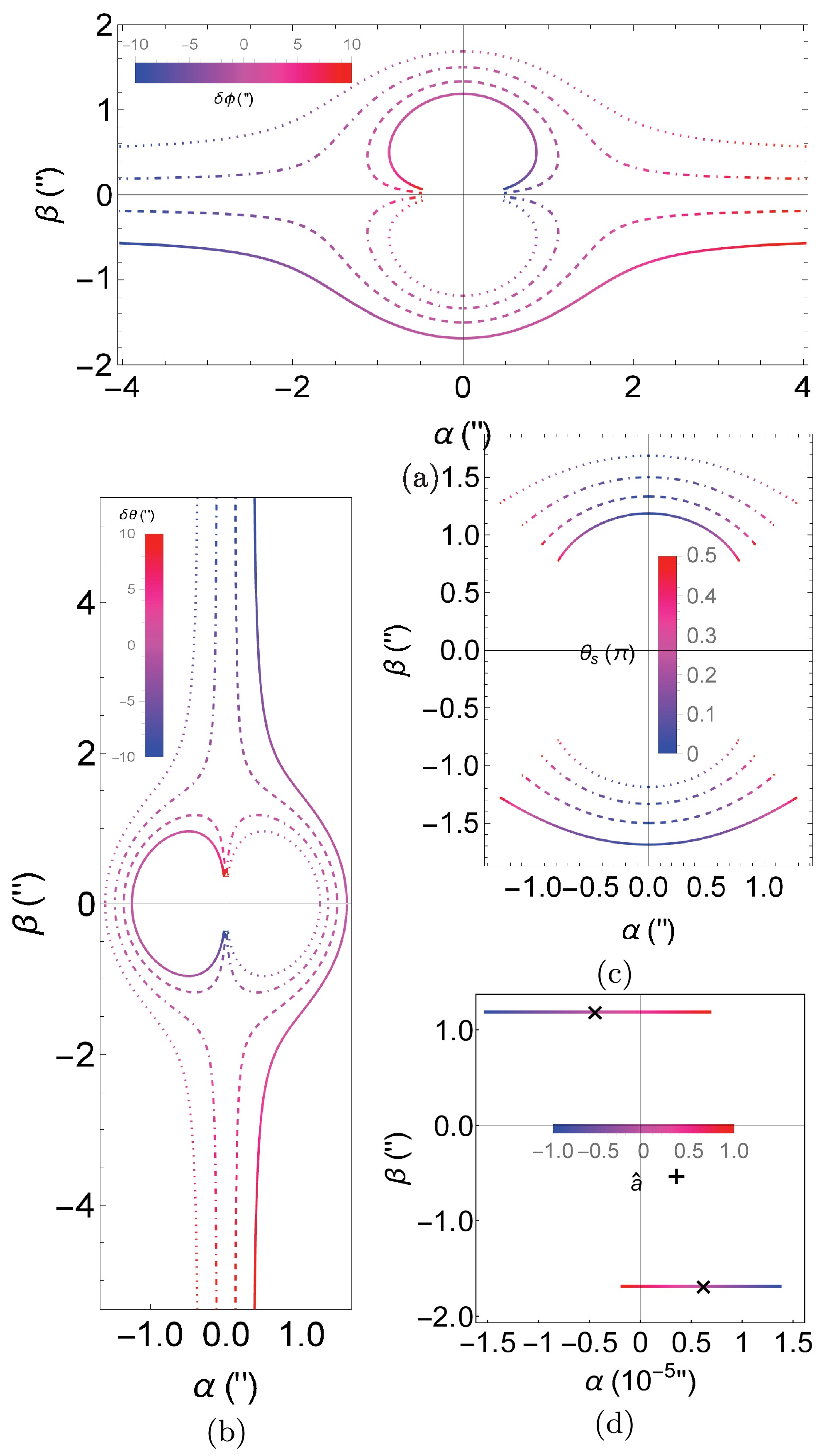

Figure 6.  (color online) Dependence of apparent angles $(\alpha,\,\beta)$ on (a) $\delta\phi$ from $-10^{\prime\prime}$ to $10^{\prime\prime}$ , (b) $\delta\theta$ from $-10^{\prime\prime}$ to $10^{\prime\prime}$ , (c) $\theta_ \mathrm{s}$ from $0.01\pi$ to $\pi/2$ , and $\hat{a}$ from -1 to 1 in (d) for $\delta\phi=5\times 10^{-6\prime\prime}$ and $\delta\theta=1^{\prime\prime}$ . The different line types in (a), (b), (c) are for different values of $\delta\theta,\,\delta\phi$ and $\delta\theta=\delta\phi$ . The solid, dashed, dot-dashed, and dotted lines represent $1^{\prime\prime},\,0.33^{\prime\prime},\,-0.33^{\prime\prime},\,-1^{\prime\prime}$ respectively. The default values of parameters in each subplot, except those varied, are $\delta\theta=1^{\prime\prime},\,\delta\phi=1^{\prime\prime},\,\hat{a}=1/2,\,r_ \mathrm{s}=r_ \mathrm{d},\,v=1$ .

on the celestial plane of the observer.

In Fig. 6 (a), we continuously vary the $\phi$ coordinate and consequently $\delta\phi$ of the source while keeping $\theta_ \mathrm{s}$ and $\hat{a}$ fixed and show the tracks of the images for several discrete $\delta\theta$ . The value of $\delta\phi$ is color-coded for the left side of the tracks to correspond to $\delta\theta=-10^{\prime\prime}$ and the right side to $\delta\theta=10^{\prime\prime}$ . For each fixed set of parameters in the selected parameter range, two conjugate images distributed in opposite quadrants always appear, on the same straight line passing the origin. For $\hat{a}=1/2>0$ and $\delta\theta>0$ , the image pairs in the first and third (or the fourth and second) quadrants are when $\delta\phi<0$ (or $\delta\phi>0$ ) and correspond to retrograde and prograde test particles, respectively. For $\hat{a}=1/2>0$ and $\delta\theta<0$ , the opposite occurs. In each pair of images, the one on the outer curves, i.e., the curves further away from the origin, has a larger minimal radial coordinate and the one on the inner circular curves has a smaller $r_0$ . For the selected parameter ranges of $\delta\theta$ and $\delta\phi$ , because the effect of $\hat{a}$ is not apparent (see Fig. 5), the lens images appear almost symmetric for $\delta\theta$ or $\delta\phi$ with opposite signs.

Among each pair of the images, we observe that for each fixed $\delta\theta$ , with decreasing $\delta\phi$ , the $\alpha$ -coordinate of the far-side image increases monotonically. Again, the reason is simply that the variation in the $\phi$ coordinate of the source is parallel to the $\alpha$ axis in the celestial plane. The qualitative characteristics of the angular locations of the inner images are more interesting. When $\delta\phi$ increases to large values, although the $\beta$ coordinates of the outer images do not approach zero, those of the inner images do. When $|\delta\phi|$ decreases from large values, the $\alpha$ coordinates of the inner images do not decrease monotonically but initially increase to a maximal value and then decrease, indicating that the effect of $\delta\phi$ begins to dominate the image locations. This last feature corresponds with Fig. 2 (c).

Figure 6 (b) shows the dependence of the image locations on $\delta\theta$ for a few fixed $\delta\phi$ . Qualitatively, this figure resembles a rotation of Fig. 6 (a), indicating that the role of $\delta\phi$ in Fig. 6 (a) is now played by $\delta\theta$ . An apparent difference is that the range of $\beta$ in Fig. 6 (b) is about $1.4\approx \sqrt{2}=1/\sin\theta_ \mathrm{s}$ times that of $\alpha$ angle in Fig. 6 (a). This is a reflection of the $\sin\theta_ \mathrm{s}$ factor in the contribution of $\delta\theta$ and $\delta\phi$ to the total deflection in Eq. (45).

In Fig. 6 (c), we illustrate the effect of $\theta_ \mathrm{s}$ on the image location while fixing $\delta\phi=\delta\theta=1^{\prime\prime}$ . We observe that when $\theta_ \mathrm{s}$ approaches the spacetime rotation axis, both images are shifted very close to the $\alpha$ axis, which is consistent with the fact that both $\theta_{ \mathrm{e}\pm}$ approach the $\hat{z}$ axis in Fig. 3 (b). However, when $\theta_ \mathrm{s}$ converts to $\pi/2$ , the images do not approach zero $\beta$ but rather a finite $\beta$ that is smaller than $\delta\theta$ . This also corresponds with the observation from Fig. 3 (b) that $\theta_{ \mathrm{e}\pm}$ approaches only some middle values not close to either 0 or $\pi/2$ . The more fundamental reason for these phenomena is simply that $\delta\theta$ is still non-zero in this case, i.e., the detector is still below the equatorial plane. Generally, the apparent angle $\gamma_\pm\approx \sqrt{\alpha_\pm^2+\beta_\pm^2}$ in this figure does not change significantly as $\theta_ \mathrm{s}$ varies, because the total effective deflection given by Eq. (45) does not change by a large factor.

For the ranges of parameters considered in Fig. 6 (a)−(c), we can easily verify that the critical scenario in which the effect of $\hat{a}$ becomes significant is never reached. Therefore, for these parameter ranges, in principle, we expect that the apparent angles can be well approximated by the results in Schwarzschild spacetime. When the source is located on the equatorial plane, the apparent angles against the lens-detector axis to the leading order are [22]

where

Here, we replaced $\delta\phi$ in the Schwarzschild spacetime with the total deflection $\delta\eta$ in the Kerr spacetime, i.e., Eq. (45). However, because the source now is not located on the equatorial plane, these images should be rotated on the celestial plane such that the trajectories are in the same plane as the source, lens, and detector. The location of the source with the absence of the lens in Eq. (50) provides for the two images rotation angle $\xi$ from the $+\hat{\alpha}$ axis on the celestial plane, i.e.,

Applying the above rotation to the apparent angles in Eq. (51), we finally determine the apparent angles $(\alpha_\pm,\,\beta_\pm)$ for sources in Kerr spacetimes with a small $\hat{a}$ as

where $\zeta$ is in Eq. (52). We replot image locations $(\alpha_\pm,\,\beta_\pm)$ using the equations provided above for parameters given in the caption of Fig. 6 (a)−(c) and observe excellent agreement with these figures. Moreover, these formulas can be used to explain the relevant results in Ref. [48].

Figure 6 (d) shows the effect of $\hat{a}$ on the apparent angles of the images. We intentionally select a small but positive $\delta\phi$ for $\hat{a}$ to pass the critical $\hat{a}_c$ discussed in Fig. 5 as it varies from $-1$ to 1. The two black crosses mark the images for $\hat{a}=0$ , and the plus sign marks the location of the source if the lens were absent. The most interesting characteristic in these plots, and in contrast to the cases in (a)−(c) where the effect of $\hat{a}$ is not evident or equivalently the Schwarzschild case, is that as $\hat{a}$ increases from zero, the retrograde (or prograde) trajectories begin to approach the $+\hat{z}$ axis (or the $-\hat{z}$ axis), and the corresponding image begins to approach the $\hat{\beta}$ axis from the left (or right). When $\hat{a}$ passes $\hat{a}_{c+}$ , the retrograde trajectory intersects the $\hat{z}$ axis first and then its image appears on the right side of the $\hat{\beta}$ axis. In other words, until $\hat{a}$ reaches $\hat{a}_{c-}$ , two prograde trajectories and images with $\alpha>0$ occur. Eventually, when $\hat{a}$ passes $\hat{a}_{c-}$ , the initially retrograde trajectory passes the $-\hat{z}$ axis and yields the image on the left side of the $\hat{\beta}$ axis. There will be one image from the prograde trajectory and one image from the retrograde trajectory again.

Magnifications

The magnification of the images is defined as the ratio between the observed image angular size to the source angular size if the lens is absent:

where $J_\pm$ is the Jacobian of the transformation from variables $(\delta\theta,\,\delta\phi)$ to $(\alpha_\pm,\,\beta_\pm)$ . This agrees with Ref. [49], which considered the (quasi-)equatorial plane case.

Using Eqs. (46a) and (46b), $(\alpha_\pm,\,\beta_\pm)$ are related to $(L,\Theta)$ , which according to Eqs. (7) and then (15) and (16), are functions of $(r_{0\pm},\,\theta_{ \mathrm{e}\pm})$ . These quantities can be finally connected to $\delta\theta$ and $\delta\phi$ through solutions of $\theta_{ \mathrm{e}\pm}$ and $r_{0\pm}$ . Therefore, using the chain rule for the partial derivatives, each element in the Jacobian can be computed as

where $y$ can be either $\theta$ or $\phi$ . Substituting $r_{0\pm}$ and $\theta_{ \mathrm{e}\pm}$ for each image into the above equation, we can immediately obtain the magnifications of the two images. We denote the magnification for the prograde image as $\mu_+$ and for the retrograde image as $\mu_-$ .

When $\delta\theta$ is large such that the effect of $\hat{a}$ is weak, then this magnification can be simplified to that of a Schwarzschild spacetime

and the total deflection $\delta\eta$ in Eq. (45) has replaced the corresponding deflection $\delta\phi$ in the Schwarzschild spacetime. From this, the effects of parameters $\delta\phi,\,\delta\theta,\,\theta_ \mathrm{s}$ are very apparent.

In Fig. 7, we show the dependence of the magnification on the parameters $\delta\phi,\,\delta\theta$ . We observe from Fig. 7 (a) that the magnifications $\mu_\pm$ for both images decrease as any of $\delta\phi$ and $\delta\theta$ increases. Moreover, the magnification $\mu_+$ of the prograde image decreases to zero, whereas $\mu_-$ of the retrograde image decreases to $1$ , which are the asymptotic values of Eq. (58). From Fig. 7 (b), we observe that when both $\delta\phi$ and $\delta\theta$ are small, both magnifications $\mu_\pm$ become very large, a characteristic qualitatively similar to the magnifications of lensed images in SSS spacetime but with the total deflection angle $\delta\eta$ in (45) playing the role of the deflection in SSS spacetime [22]. However, we observe from the peak in Fig. 7 that the value of $(\delta\theta,\,\delta\phi)$ for which the magnifications diverge fastest do not occur when $\delta\theta\to 0$ . This can be attributed to the effect of the spacetime spin.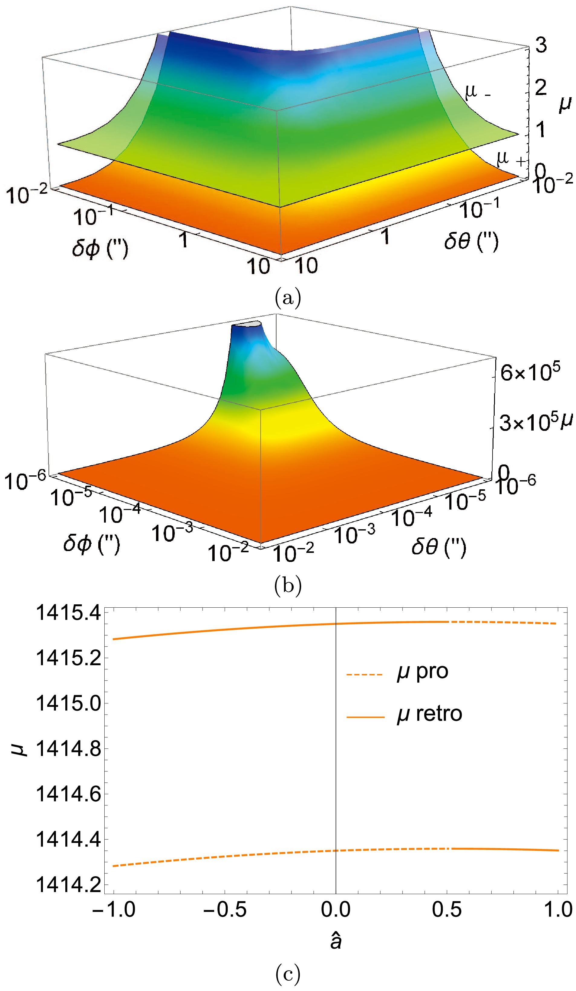

Figure 7.  (color online) Dependence of the magnification on $\delta\phi$ and $\delta\theta$ (a) and (b) and on $\hat{a}$ (c). We fix $\hat{a}=1/2$ in plots (a) and (b) and $\delta\phi=5\times 10^{-6\prime\prime},\,\delta\theta=10^{-3\prime\prime}$ in (c). Other parameters are $\theta_ \mathrm{s}=\pi/4,\,r_ \mathrm{s}=r_ \mathrm{d},\,v=1$ .

In Fig. 7 (c), we show the effect of $\hat{a}$ on magnification is shown. A small $\delta\phi$ is selected for the effect of $\hat{a}$ to be apparent. Generally, for a positive $\delta\phi$ , $\mu_\pm$ increases with the increase in $\hat{a}$ up to approximately the critical values $\hat{a}_{c\pm}$ . Thereafter, the magnification decreases. The magnification around $\hat{a}_{c\pm}$ being maximal for each trajectory can be qualitatively understood from the fact that the trajectory is often closer to the lens than other $\hat{a}$ around this spin.

To determine the time delay between the two lensed images, we must first compute total travel time $\Delta t$ along the two trajectories. This can be performed completely in parallel to the computation of deflection angle $\Delta\phi$ in Secs. II and III. Because the computation and presentation therein are quite lengthy, we will address the total travel time and time delay separately here.

Starting from Eq. (5d), and using Eqs. (5a) and (9) in the first and last terms in the right-hand side of this equation, respectively, it becomes

The procedure to compute perturbative $\Delta t$ is then the same as that from Eqs. (10) to (30) for $\Delta \phi$ . The result is

where $H_{r,i}$ and $H^{\prime}_{\theta,i}$ are analogous to $G_{r,i}$ and $G^{\prime}_{\theta,i}$ in Eq. (26e)−(26d). Their first few orders are

where $p_j,\, a_1$ are given in Eqs. (18) and (29a), respectively.

The null limit of $\Delta t$ can be obtained easily by taking $v=1$ in the above equation:

We have also checked that $\Delta t$ in Eq. (61) can reduce to its equatorial plane form computed from Eq. (53) of Ref. [14] if we let $\theta_ \mathrm{s}\to\pi/2,\,\theta_ \mathrm{e}\to\pi/2$ .

The $\Delta t$ above can be further expanded in the small $p_\mathrm{s,d}$ limit. The result to the first few orders is determined to be

where the coefficients are

This $\Delta t$ is a function of $r_0$ and $\theta_e$ . Therefore, when these two quantities, as well as other parameters determining them, are known for a given trajectory, the corresponding $\Delta t$ will be fixed. For the two images formed from the same source but with different $r_{0\pm}$ and $\theta_{ \mathrm{e}\pm}$ , time delay $\Delta^2 t_\pm\equiv \Delta t_+-\Delta t_-$ can be derived through straightforward deduction. Using Eq. (64), we determine $\Delta^2 t_\pm$ to the leading three orders as

We observe that the dominant term (Eqs. (65a)) in Eq. (64) does not contribute to the time delay because it is the time corresponding to the straight line approximation and is the same for both trajectories. The terms retained in this analysis originate from Eqs. (65b), (65c), (65f), and (65d). The effects of spacetime spin and non-equatorial effects are present in the terms from Eq. (65f).

In Fig. 8, we plot the dependence of the time delay $\Delta^2 t_\pm$ on $\hat{a}$ for a source with $\delta\phi=4^{\prime\prime}$ and $\delta\theta=1^{\prime\prime}$ , and the lens is still assumed to be Sgr A*. Because $\delta\phi$ is very small, as indicated in Fig. 5 and revealed in Ref. [14], the spin $\hat{a}$ is expected to have a significant impact on the time delay. Thus, as $\hat{a}$ varies from $-1$ to 1, the time delay changes from approximately $0.025$ s to $0.83$ s. The time delay reaches its minimum value at approximately $\hat{a} = 0.11$ , which is close to the critical value $\hat{a}_{c\pm}$ . In other regions, the time delay varies with approximately a constant size but appreciable slope.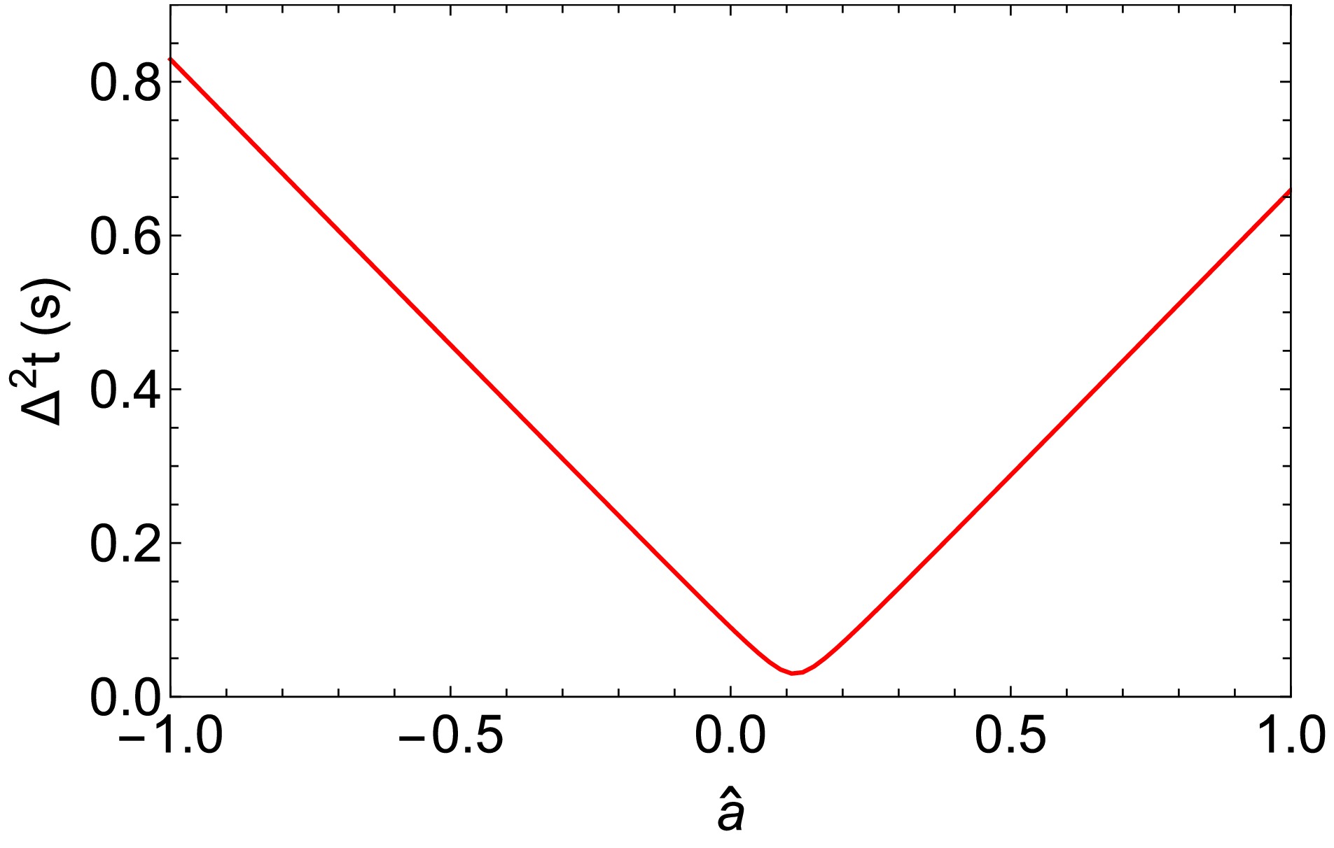

Figure 8.  (color online) Dependence of the time delay $\Delta^2 t_\pm$ on $\hat{a}$ for $\delta\phi=4^{\prime\prime}\; ,\delta\theta=1^{\prime\prime},\,r_ \mathrm{s}=r_{s_{39}}=5672.6511(M),\,\theta_ \mathrm{s}=\pi/4,\,v=1$ .

In this section, we discuss a few problems that our results can be used to study.

We first study the images of a source moving in the equatorial plane behind the lens. Such sources can include stars or other transits whose orbit (almost) intersect with the observer-lens axis and whose angular velocity is appreciable to make the observation of the motion possible, e.g., some S stars around Sgr A*.

In Fig. 9, we assume that the source is located at a representative radial distance of the S star orbits and plot the location of the GL image of this source as it moves across. Because we are working within a WDL, the section of the trajectory that we can treat appears almost a straight line if no lens exists. We assume that this straight line satisfies the parametric relation $\delta\phi=\delta_0+\delta\theta$ where $\delta_0$ takes on a few values of $10^{-5\prime\prime},10^{-3\prime\prime},10^{-1\prime\prime}$ and $\delta\theta$ runs from $-10^{\prime\prime}$ to $10^{\prime\prime}$ in Fig. 9 to compute the corresponding image locations.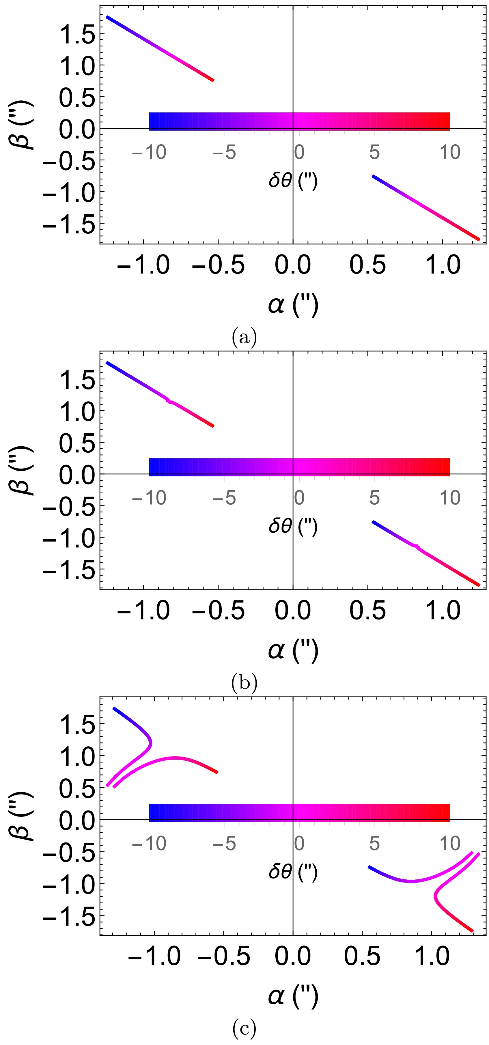

Figure 9.  (color online) Dependence of the apparent image and magnification on moving sources, where $\delta\phi=\delta_0+\delta\theta$ and $\delta\theta$ from $-10^{\prime\prime}$ to $10^{\prime\prime}$ . We fix $\hat{a}=1/2,\theta_ \mathrm{s}=\frac{\pi}{4},\,r_ \mathrm{s}=r_ \mathrm{d},\,v=1$ and $\delta_0=10^{-5\prime\prime}$ (a), $\delta_0=10^{-3\prime\prime}$ (b), $\delta_0=10^{-1\prime\prime}$ (c).

When $\delta_0$ is relatively small, i.e., for the $\delta_0= 10^{-3\prime\prime},\,10^{-5\prime\prime}$ cases, the images of a source moving along a straight line in the backend also form two straight tracks on the celestial sphere. This indicates that in this parameter setting, the effect of the spacetime spin is not important in determining the apparent angles of the images. However, when $\delta_0$ is larger (i.e., $10^{-1^{\prime\prime}}$ ), the image tracks deviate from straight lines at some point of $\delta\theta$ or $\delta\phi$ . This is indeed the value of $\delta\theta$ and $\delta\phi$ such that the critical $a_c=1/2$ , which is the value we set for the spacetime spin when plotting this figure. This sharp derivation from straight lines of the tracks can be used as a characteristic observable of $a_c$ .

Among possible sources lensed by a Kerr BH, stars or other spherical shape objects are very natural candidates. If the source and/or the lens are small and too far from us such sthat the shape of the images are not resolvable, then only the central values of the apparent angles $(\alpha,\,\beta)$ might be obtained. However, when the source is large or close and the detector has sufficient resolution, the shape of the source should also be recognizable. Thus, in an SSS spacetime, we would expect that the images of a spherical source will generally appear elongated.

In the Kerr spacetime, if $\delta\theta$ and $\delta\phi$ are sufficiently large that the effect of $\hat{a}$ is much weaker on the trajectory deflection, then naturally we would expect that the shape of the images will be similar to those in the Schwarzschild spacetime with $\delta\eta$ in Eq. (45) playing the role of the source's deflection. In this case, we can determine the shape of the images based on the apparent angle formula (51) in the Schwarzschild spacetime. If the radial coordinate of the source object is $R$ , where $R/r_ \mathrm{s}\ll \delta\eta$ (see Fig. 10), and denoting the polar angle of a boundary point of the source as $\sigma$ in a polar frame with the center of the source at the origin, then to this leading order of $R/r_ \mathrm{s}$ , the total deflection angle of this boundary point with respect to the Schwarzschild lens becomes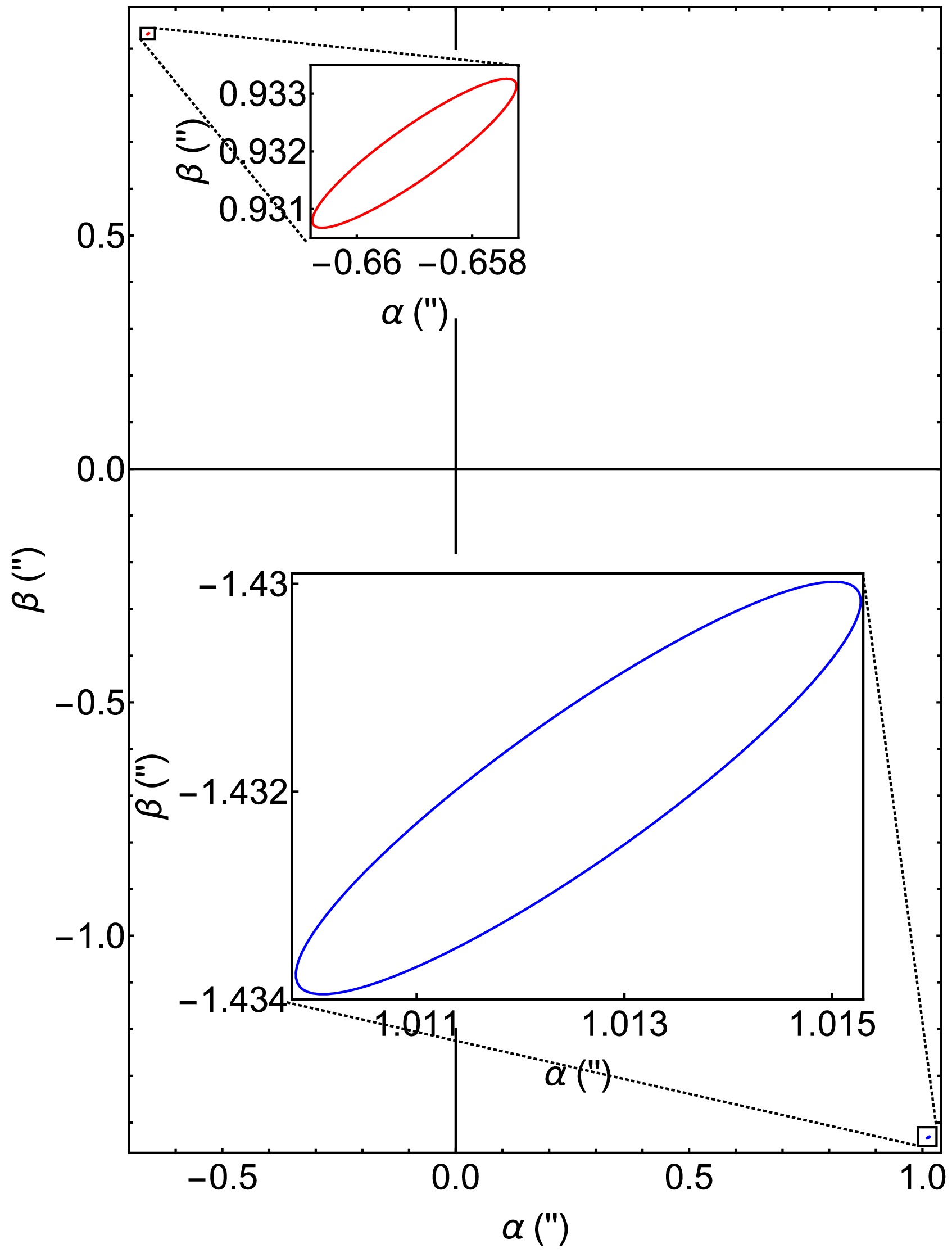

Figure 10.  (color online) Apparent angles $(\alpha,\,\beta)$ of the two images of a star with twice the Sun's size. We fix $s_{r\theta}=+1,\,s_{l}=+1,\,\theta_ \mathrm{s}=\pi/4,\,\delta\phi=\delta\theta=1^{\prime\prime} ,\,\hat{a}=1/2,\,r_ \mathrm{s}=r_ \mathrm{d},\,v=1$ . The red, blue, and black dashed lines are the two lensed images and the source shape without the presence of the lens (the insets are the magnified images).

Substituting this into Eq. (51) and to the first order of $R/r_ \mathrm{s}$ , the boundaries of the two images now have apparent angles $(\alpha_{S,\pm}^\prime,\,\beta_{S,\pm}^\prime)$ with

where $\alpha_{S,\pm}$ is in Eq. (51) and $\zeta$ in Eq. (52). The last term is the small variation $\delta\alpha_{\pm}$ of the apparent angle in the $\alpha$ direction of the images. Similarly, the extension of the images in the $\beta$ direction is

Equations (68) and (69) clearly demonstrate that the images on the celestial sphere have elliptic shapes with $\delta\alpha_{\pm}$ and $\delta\beta_{\pm}$ being the semi-minor and semi-major axes, respectively, with the semi-minor axis aligned with the image-lens axis. The eccentricity of these ellipses are

The corresponding magnifications of the images are the ratio between the angular size of the images and the original source

We can check that this agrees with the magnification (58) for images of the source at $\delta\eta$ .

In Fig. 10, we show the image locations of a star with twice the size of our Sun and located at $r_ \mathrm{s}=100^{\prime\prime}r_ \mathrm{d}$ and $\delta\theta=\delta\phi=1^{\prime\prime}$ . We observe that they do take the elliptic shape, and we have checked that their eccentricity and magnifications match exactly the values specified by Eqs. (70) and (71).

Kerr BH spacetime is considered the most important BH in astronomy, whereas SMBH Sgr A* is currently one of the best confirmed BH candidates. Even being so close to us, Sgr A* still has many properties not well-constrained, including its spin orientation against our line-of-sight.

However, if the images of a source that is well aligned with the detector-lens axis are observed, then we might attempt to constrain the inclination of the spin, which is given by $\theta_i=\pi/2-\theta_s$ in this case. Among input parameters $\{M,\,a,\,\theta_ \mathrm{s},\,r_ \mathrm{s},\,r_ \mathrm{d},\,\delta\theta,\,\delta\phi, \; v\}$ , parameters $M,\,\hat{a}$ , and $\theta_ \mathrm{s}$ are associated with the BH itself. Parameters $r_ \mathrm{s},\,\delta\theta$ , and $\delta\phi$ are associated with the source and $r_ \mathrm{d},\,v$ are associated with the detector and test particles, respectively. Generally, parameters $M, \; r_ \mathrm{d}$ can be obtained through other means and we can set $v=1$ for photons. $\delta\theta,\,\delta\phi$ generally cannot be measured, whereas $r_ \mathrm{s}$ can occasionally be deduced from the spectrum redshift if the source is a far-away galaxy but would be more difficult to measure for a typical star in the Galaxy. The spin of Sgr A* has been measured although not tightly [50]; therefore, in this paper, we primarily attempt to constrain its orientation against the line-of-slight.

We assume that for a GL scenario by a Kerr BH, we can observe either the angle $\sigma$ between the line connecting the two images and the projection of $\hat{a}$ on the celestial sphere, i.e.,

or the time delay $\Delta^2 t_\pm$ between the two images. Each of these two quantities enable us to solve $\theta_s$ and consequently the inclination $\theta_i$ . We have listed a few typical values of the observed $\sigma$ or $\Delta^2t_\pm$ and the deduced $\theta_i$ in Table 1. We observe that $\theta_i$ depend on $\sigma$ and $\Delta^2 t_\pm$ very sensitively and therefore can be well constrained by them.

$\Delta^2 t_\pm$ /s	$\theta_i$ /rad	$\sigma$ /rad	$\theta_i$ /rad
0.2	1.31	0.05	0.67
0.3	1.17	0.10	1.17
0.4	1.02	0.15	1.31
0.5	0.86	0.20	1.38
0.6	0.67	0.25	1.42

Table 1.  Deduction of BH spin inclination $\theta_i=\pi/2-\theta_s$ from $\Delta^2t$ or $\sigma$ . Columns 1 and 3 are assumed measurements and columns 2 and 4 are solved $\theta_i$ . We fix $\delta\theta=1^{\prime\prime}, \; \delta\phi= 10^{-5\prime\prime} ,$ $r_ \mathrm{s}=r_{s39},\,v=1,\, \hat{a}=0.7$ .

This work considers the deflections and GL of both null signals and massive particles in the off-equatorial plane in Kerr spacetime in the WDL. The deflection angles are computed using the perturbative method resulting in power series expansions of $M/r_0$ and $r_0/r_{\mathrm{s,d}}$ , with the coefficients being functions of the spacetime parameter and the trigonometric function of the extreme values $\theta_ \mathrm{e}$ along the trajectories. Moreover, the finite distance effect of the source and detector is considered in these deflections. This enables us to establish a set of exact GL equations, from which we can solve the desired $(r_0,\theta_ \mathrm{e})$ , enabling the test particle from a source with deviation angles $\delta\theta$ and $\delta\phi$ to reach the detector.

Using the exact formula for the apparent angles derived for the off-equatorial plane test particles, we studied the effect of various parameters, including source deviation angles $\delta\theta$ and $\delta\phi$ and spacetime spin $\hat{a}$ and its orientation $\theta_ \mathrm{s}$ , on the angular locations of the images on the celestial sphere and their magnifications. Generally, two trajectories that will reach the detector exist. For given values of $\delta\theta$ and $\delta\phi$ , two critical values of $\hat{a}_c$ at which the two test particles intersect the positive and negative $\hat{z}$ directions, respectively, always exist. Generally, when $\delta\theta$ or $\delta\phi$ is large, the effect of $\hat{a}$ (for the Kerr BH $\hat{a}\leq1$ ) becomes subdominant; therefore, the GL is approximately the same as that in Schwarzschild spacetime (but in the off-equatorial plane). However, in other cases, $\hat{a}$ will affect the quadrant in which the images appear and the magnification of these images.

We also obtained the time delays between the two images. We found that the time delay generally depends on spacetime spin $a$ very sensitively even when deviation angles $\delta\theta$ and $\delta\phi$ are not very small. Therefore, it can be used as an effective tool to constrain $a$ , as was demonstrated in an equatorial case [14].

We used these results to study the image of a transiting source behind the lens and the image shape and size of a spherical source, and we used the observables to deduce properties of the BH and its orientation.

A few points must be mentioned here. First, although this work primarily studies the BH spacetime with $|a|\leq M$ , it is not restricted to this range. Therefore, the method and results can be applied to the naked singularity case. Second, from the mathematical perspective, the perturbation method should be generalizable to the deflection and GL in the off-equatorial plane of other axisymmetric spacetime. We will report the findings along this direction in a follow-up work.

In this appendix, we show that the integrals of the forms (22) and (23) can always be determined and the results are elementary functions.

For the integral (22), multiplying the numerator and denominator of the integrand by $(1-p)^{i-1}$ , the integral is transformed to the sum of integrals of the form of the left-hand side of the following equation:

where the integration is performed by parts. Note that, superficially, the first term on the right-hand side might diverge when $p$ approaches $1$ . However, all these divergences will cancel when substituting these results into Eq. (22) because this is an artifact introduced when multiplying its integrand denominator by $(1-p)^{i-1}$ . The recursion relation (A1) enables us to lower the order of the numerator by 2. Finally, for the lowest two orders $k=0,\,1$ cases, we have

From the above relations, we observe that the result of integration (22) is a sum of terms such as $p^m/(1-p^2)^{n-1/2}\; (m,n=1,2,\cdots)$ , which are elementary functions.

For integral (23), using a further change of variable $x=c/c_ \mathrm{e}$ , after integration by parts and simplification, it becomes

Using this recursion relation and the lowest order integral

we observe that (23) can also be completely integrated and the result is a sum of elementary functions.

In this appendix, we present two approaches for the derivation of $\cos(\theta_ \mathrm{d})$ in terms of other kinematic parameters. The resultant Eq. (27) will act as one of the two GL equations from which $\theta_ \mathrm{e}$ and $r_0$ can be solved. The first approach is the Jacobian elliptic function method, which directly solves Eq. (11) for $\cos\theta_ \mathrm{d}$ . The second approach uses the method of undetermined coefficients.

For the first method, inspecting Eqs. (6) and (7) and focusing on their dependence on $c$ and $r$ respectively, we can factor them as

where $c_ \mathrm{e}$ and $r_0,\,r_1,\,r_2,\,r_3$ are the roots of $\Theta(c)=0$ and $R(r)=0$ , respectively, and we order them as $r_0>r_1>r_2>r_3$ . Coefficients $B_0$ and $B_1$ are

With this re-writing, Eq. (9) can be solved to determine a solution of $\cos(\theta)$ as a function of $r$

where $\mathrm{cn}(x|y)$ is the Jacobian elliptic function, $C$ is the integral constant, and

where $F_1(x|y)$ is the elliptic integral of the first kind.

To fix constant $C$ , we use boundary condition $\theta(r=r_ \mathrm{s})=\theta_ \mathrm{s}$ to determine

where the $-$ and $+$ signs in $\mp$ correspond to the branch of trajectory from $r_ \mathrm{s}$ to $r_0$ and from $r_0$ to $r_ \mathrm{d}$ , respectively. Substituting Eq. (B4) and $r=r_ \mathrm{d}$ into solution (B3) and expanding the result in terms of small $M/r_0$ , we obtain series (27).

In the second method to determine the relation between $c_ \mathrm{d}$ and $r_0$ , we start by assuming that $c_ \mathrm{d}$ takes a series form as in Eq. (27) and then use the method of undetermined coefficients to determine these $h_i$ values.

Substituting this series form into the right-hand side of Eq. (24) and then recollecting the series according to the power of $(M/r_0)$ , we obtain

where the first few $F_{\theta,i}^\prime$ are listed as

Coefficients $h_i$ here can be fixed by comparing with the left-hand side of Eq. (24) for the coefficient of $(M/r_0)^n$ order by order, i.e.,

Fortunately, this set of systems can be solved iteratively because $h_i$ always starts to appear from $F_{\theta,i+1}^\prime$ and the equation system is sufficiently simple. The result of the solutions to $h_i$ are exactly Eq. (28c).

First, we denote the four-velocity of the test particle and a direction between which we seek to measure the angle as $v^\mu$ and $k^\mu$ , respectively; thus, we have

For $k^\mu$ , we have three natural choices: directions $\hat{r}_ \mathrm{d},\,\hat{\theta}_ \mathrm{d}$ , and $\hat{\phi}_ \mathrm{d}$ , which are the spacelike directions of tetrad $e^\mu_{(a)}$ associated with a static observer with four-velocity $u^\mu$

For such static observers, we can use projection operators

to project each of the test particle or directional vectors $v^\mu,\; \hat{r}_ \mathrm{d},\,\hat{\theta}_ \mathrm{d},\,\hat{\phi}_ \mathrm{d}$ into a spacial part and a temporal part in the rest frame of the observer, respectively [51]:

Thus, the apparent angle of the signal against $\hat{r}_ \mathrm{d}$ is given by

and the angles between the signal and the $\hat{r}_ \mathrm{d}\hat{\theta}_ \mathrm{d}$ plane and the $\hat{r}_ \mathrm{d}\hat{\phi}_ \mathrm{d}$ plane are respectively

Substituting the Kerr metric, we can determine the expressions for these three angles as