Pole determination of $ {\boldsymbol X{\bf{(3960)}}} $ and $ {\boldsymbol X_{\bf 0}{\bf{(4140)}}} $ in the decay ${{\boldsymbol B}^{\bf +}{\bf\to}{\boldsymbol D}_{\boldsymbol s}^{\bf +}{\boldsymbol D}_{\boldsymbol s}^{\bf -}{\boldsymbol K}^{\bf +} }$

For a long time, we have been asking the question, "What type of matter can be formed by quark models?" The traditional quark model successfully explains that baryons are complexes of three quarks and mesons are combinations of quarks and antiquarks. With the advancements in experimental methods, the recent discovery of candidates for the pentaquark and tetraquark states in experiments has expanded the scope of our study of traditional hadrons, which include qualitatively different $ qqq\bar{q}\bar{q} $ and $ qq\bar{q}\bar{q} $. In addition, more exotic structures have been observed in experiments; see Refs. [1−8]. To answer the appeal question, we must determine whether the pentaquark and tetraquark states exist.

In determining the strange state of quantum chromodynamics (QCD), the decay process of B mesons will be an important and effective platform. In this process, many candidates for strange hadron states can be observed. Over the past few years, major laboratories have successively discovered candidates for strange hadron states in the decay of B mesons, such as $ Z_{cs}(4000) $ and $ Z_{cs}(4000) $ [9], $ X(4140) $ [10, 11] in $ B^+\to J/\psi\phi K^+ $, and $ X_0(2900) $ and $ X_1(2900) $ in $ B^+\to D^+D^-K^+ $ decay [12, 13]. Referring to these experiments, we can observe that the three-body decay of B mesons can provide much information on hadron resonance; see Refs. [14−17].

Very recently, the LHCb Collaboration reported a new near-threshold structure named $ X(3960) $ in the $ D_s^+D_s^- $ invariant mass distribution of the decay $ B^+\to D_s^+D_s^-K^+ $. The peak structure is very close to the $ D_s^+D_s^- $ threshold with a statistical significance larger than 12σ. The mass, width, and quantum numbers of this structure were measured to be $ M=3956\pm5\pm10 $ MeV, $ \Gamma=43\pm13\pm8 $ MeV, and $ J^{PC}=0^{++} $. The LHCb analysis indicates that this structure is an exotic candidate consisting of $ cs\bar{c}\bar{s} $ constituents. In addition, when checking the data of the $ D_s^+D_s^- $ invariant mass distribution, a dip is observed at approximately $ 4.14 $ GeV; the LHCb interpreted it as another structure named $ X_0(4140) $ with a mass of $M= 4133\pm6\pm6$ MeV, width of $ \Gamma=67\pm17\pm7 $ MeV, and quantum numbers of $ J^{PC}=0^{++} $ [18]. As analyzed by the LHCb Collaboration, $ X_0(4140) $ might be caused by either a new resonance with the $ 0^{++} $ assignment or a $ D_s^+D_s^-J/\psi\phi $ coupled-channel effect, but no firm conclusion has been reached [18].

Many theoretical studies have shown much interest in X resonances. In recent years, many studies have used different models and technical methods to analyze the characteristics of exotic mesons $ cs\bar{c}\bar{s} $ [19−26]. To determine the origin and structure of $ X(3960) $ in decay $B^+\to D_s^+D_s^-K^+$, scholars have proposed many explanations for the possibility of this structure. Because its mass is close to the $ D_s^+D_s^- $ threshold, this structure can be interpreted as a possible hadronic molecule. Refs. [27, 28] proposed to treat $ X(3960) $ as the molecular state of $ D_s^+D_s^- $ with $ J^{PC}=0^{++} $ in the QCD sum rules approach. Another calculation with QCD two-point sum rules [29] results in the assignment that $ X(3960) $ is a scalar diquark-antidiquark state. The calculations in the one-boson-exchange model [30] also favor the molecule interpretation. It can also be analyzed through the characteristics of $ X(3960) $ using the coupled-channel method. The authors of Ref. [31] performed a coupled-channel calcuation of the interaction $ D\bar{D}-D_s^+D_s^- $ in the chiral unitary approach and interpreted $ X(3960) $ as a hadronic molecule in the coupled $D\bar{D}- D_s^+D_s^-$ system [31−33]. The author of Ref. [34] interpreted $ X(3960) $ as a $ cs\bar{c}\bar{s} $ state, whereas in Ref. [35], $ X(3960) $ was interpreted as $ 0^{++} $ $ cs\bar{c}\bar{s} $ tetraquark states using an improved chromomagnetic interaction model. In addition, another study suggested that $ X(3960) $ probably has the mixed characteristics of a $ c\bar{c} $ confining state and $ D_s\bar{D}_s $ continuum [36]. Some theoretical and experimental research has been conducted on $ X_0(4140) $, but its origins are still debated. For instance, in Ref. [35], $ X_0(4140) $ was also interpreted as $ cs\bar{c}\bar{s} $ tetraquak states. The discussion about mass and width in Ref. [29] enabled us to consider that the model is also acceptable. Because different computational models suggest different explanations, forming with new concepts and insights into this state can aid us in further understanding the origin of $ X_0(4140) $.

In this study, we analyzed the decay process $ B^+\to D_s^+D_s^-K^+ $ as published by the LHCb Collaboration. We simulated a coupled-channel model to analyze the data [37] using the default model and fitting the $ M_{D_s^+D_s^-} $, $ M_{D_s^+K^+} $, and $ M_{D_s^-K^+} $ of these three different invariant mass distributions. Using the amplitude provided by the coupled channel model, we address the following problems: (i) the pole position of $ X(3960) $ and $ X_0(4140) $ and (ii) whether the production of $ X(3960) $ is solely due to a kinematic effect.

The LHCb data reveal visible $ X(3960) $ and $ X_0(4140) $ structures around the $ D_s\bar{D}_s $ and $ D_s^{\ast}\bar{D}_s^{\ast} $ thresholds, respectively. Thus, we can reasonably assume that the structures are caused by the threshold cusps that are further enhanced or suppressed by hadronic rescatterings and the associated poles [37, 38]; see Fig. 1(a). Meanwhile, for the two peaks at 4260 and 4660 MeV, we refer to the suggestions given by the LHCb Collaboration and add two Breit-Weigner effects, as shown in Fig. 1(c). We assume that other possible mechanisms are absorbed by the direct decay mechanism in Fig. 1(b).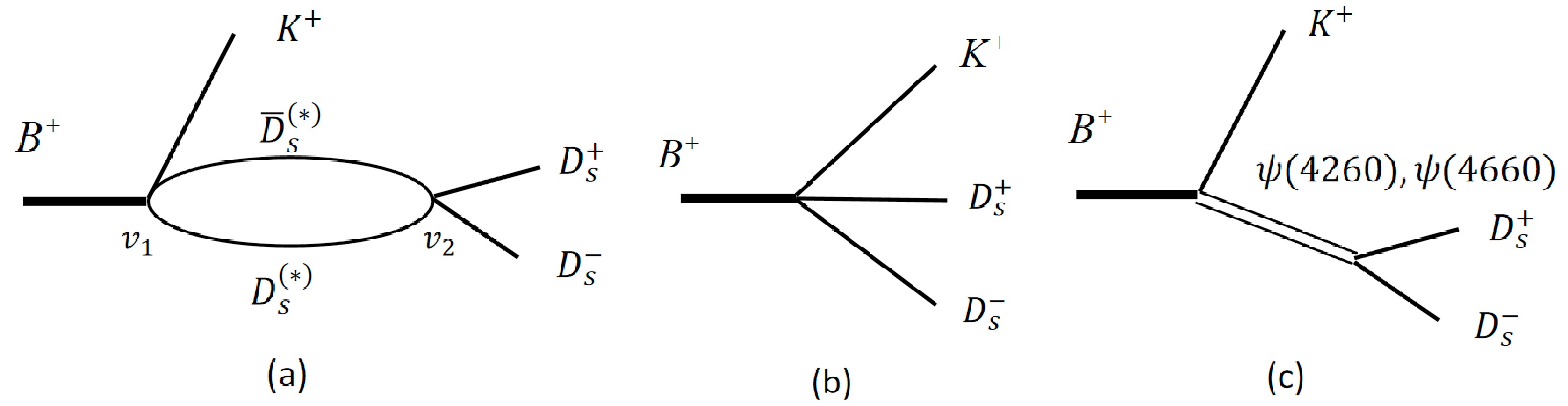

Figure 1.  Contributions of three mechanisms in the decay $ B^+\to D_s^+D_s^-K^+ $. (a) Coupled-channel; (b) Direct production; (c) Breit-Weigner effects.

First, we present the amplitude for Fig. 1(a). The first vertex $ v_1 $ is a weak interaction, and the initial weak $ B^+\to D_s\bar D_sK^+ $ vertex is

For the vertex of process $ B^+\to D_s^{\ast}\bar D_s^{\ast}K^+ $, there are two cases of parity conservation and parity violation. For the former, the vertex of $ B^+(0^-)\to D_s^*\bar{D}_s^*(0^+)K^+(0^-) $ is

in the latter case, the vertex of $ B^+(0^-)\to D_s^*\bar{D}_s^*(1^+)K^+(0^-) $ is

The energy, momentum, and polarization vector of a particle x are denoted by $ E_x $, $ \mathit{\boldsymbol{p}}_x $, and $ \mathit{\boldsymbol{\epsilon}}_x $ , respectively, and particle masses are obtained from Ref. [39]. $ c_{\alpha,B^+K+} $ is a complex coupling constant, which reprensnt $ c_{D_s\bar{D}_s,B^+K+} $ and $ c_{D_s^{\ast}\bar{D}_s^{\ast},B^+K+} $. We introduce the form factors $ f_{ij}^L $ and $ F_{kl}^L $, defined by

where $ q_{ij} $ is the momentum of i in the $ ij $ center-of-mass frame, and $ \tilde{p}_{k} $ is the momentum of k in the total center-of-mass frame. Λ is a cutoff, and $ \Lambda=1 $ GeV. We use a common value of the cutoff for all the interaction vertices.

The second vertex $ v_2 $ is hadron scattering; the perturbative interactions for $ D_s\bar{D}_s(D_s^{\ast}\bar{D}_s^{\ast})\to D_s\bar{D}_s $ are given by s-wave separable interactions. For $D_s\bar{D}_s(0^+)\to D_s^+D_s^-(0^+)$,

and for $ D_s^*\bar{D}_s^*(0^+)\to D_s^+D_s^-(0^+) $,

Another vertex exists between the two vertices, which is the coupling of the two loops, which we denote as $ v_3 $. The coupling of different loops is similar in form; for $ D_s(0^-)\bar{D}_s(0^-)\to D_s(0^-)\bar{D}_s(0^-) $,

for $ D_s(0^-)\bar{D}_s(0^-)\to D_s^*(1^-)\bar{D}_s^*(1^-) $,

for $ D_s^*(1^-)\bar{D}_s^*(1^-)\to D_s(0^-)\bar{D}_s(0^-) $,

and for $ D_s^*(1^-)\bar{D}_s^*(1^-)\to D_s^*(1^-)\bar{D}_s^*(1^-) $,

We introduce $ [G^{-1}]_{\beta\alpha}(E)=[\delta_{\beta\alpha}-h_{\beta,\alpha}\sigma_\alpha(E)] $, where $ h_{\beta,\alpha} $ is a coupling constant, and α and β are label interaction channels, with

With the above ingredients, the amplitudes for the Fig. 1(a) are respectively given by

Regarding the direct decay mechanism of Fig. 1(b),

Finally, we consider the Breit-Weigner mechanism of Fig. 1(c):

where $ \vec{p}_{K^+} $ is the $ B^+ $ CM, and $ \vec{p}_{D_s^+} $ is the $ D_s^+D_s^- $ CM; the form factor defined by

with constants $ c_{\psi(4260)} $ and $ c_{\psi(4660)} $.

We simultaneously fit the invariant mass distributions of $ M_{D_s^+D_s^-} $, $ M_{D_s^+K^+} $, and $ M_{D_s^-K^+} $ from the LHCb Collaboration using the amplitudes of Eq. (14). The amplitude includes the vertices of the weak interaction and the adjustable coupling constant resulting from the hadron interaction; this includes $ c_{D_s\bar{D}_s,B^+K^+} $, $ c_{D_s^{\ast}\bar{D}_s^{\ast},B^+K^+} $, $ c_{\psi(4260)} $, $ c_{\psi(4660)} $, $ h_{D_s\bar{D}_s,D_s\bar{D}_s} $, $ h_{D_s\bar{D}_s,D_s^{\ast}\bar{D}_s^{\ast}} $, $ h_{D_s^{\ast}\bar{D}_s^{\ast},D_s\bar{D}_s} $, and $ h_{D_s^{\ast}\bar{D}_s^{\ast},D_s^{\ast}\bar{D}_s^{\ast}} $. To reduce the number of fitting parameters, we set $ h_{D_s\bar{D}_s,D_s^{\ast}\bar{D}_s^{\ast}}=h_{D_s^{\ast}\bar{D}_s^{\ast},D_s\bar{D}_s} $, as making them different does not significantly affect the quality of the fit. Because the coupling and interaction constants of hadron scattering are consistent, we can further reduce the fitting parameters. Finally, because the magnitude and phase of the full amplitude are arbitrary, our default model has a total of nine fitting parameters. Our default model has a total of 8 (7+1) fitting parameters, in addition to these seven parameters as constants, the last parameter added is the overall factor. The parameters obtained from the final fit are shown in Table 1.

$ c_{D_s\bar{D}_s,B^+K+} $	−0.07+0.23i	−0.39+0.45i
$ c_{D_s^{\ast}\bar{D}_s^{\ast},B^+K+} $	−0.13+0.09i	−0.01+0.58i
$ c_{\psi(4260)} $	2.26−2.46i	8.21−0.77i
$ c_{\psi(4660)} $	−3.27+5.30i	−8.98−13.08i
$ h_{D_s\bar{D}_s,D_s\bar{D}_s} $	13.18+5.94i	3.83+16.02i
$ h_{D_s^{\ast}\bar{D}_s^{\ast},D_s^{\ast}\bar{D}_s^{\ast}} $	−17.10+18.21i	0
$ h_{D_s^{\ast}\bar{D}_s^{\ast},D_s\bar{D}_s} $	−15.14−11.10i	−1.47+10.20i
Λ/MeV	1000 (fixed)	1000 (fixed)

Table 1.  Parameter values for $ B^+\to D_s^+D_s^-K^+ $ models. The second and third columns are for the default and no couple-channel effect models.

We show the default model by the solid blue curves in Fig. 2, which closely matches the LHCb data. We can clearly observe the peak at 3960 MeV and a dip at 4140 MeV. The fitting quality is $ \chi^2 $/ndf=(55.67+44.66+56.08)/(127－8)$ \simeq $1.31, where three $ \chi^2 $ values result from three different distributions; "ndf" is the number of bins (43 for $ D_s^+D_s^- $, 42 for $ D_s^+K^+ $, and 42 for $ D_s^-K^+ $) subtracted by the number of fitting parameters.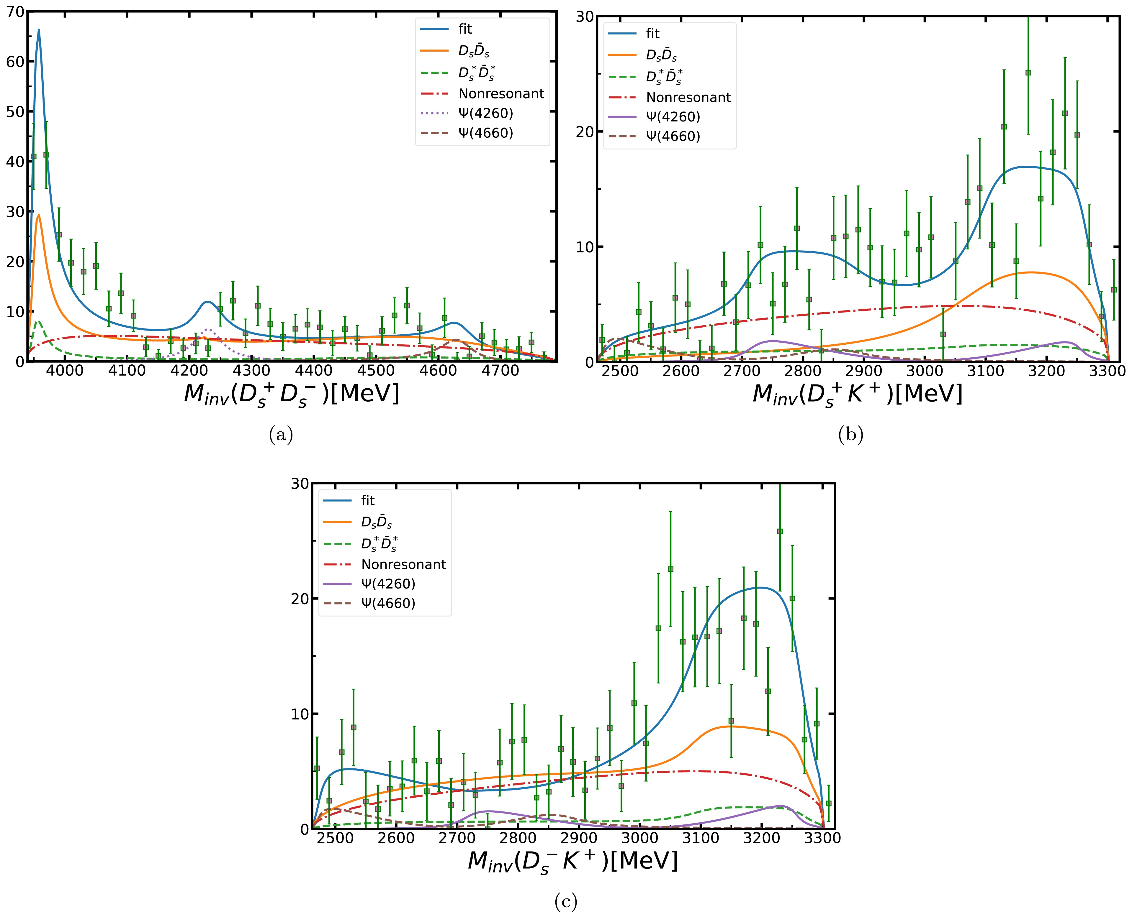

Figure 2.  (color online) (a)$ D_s^+D_s^- $, (b)$ D_s^+K^+ $, (c)$ D_s^-K^+ $ invariant mass distributions for $ B^+\to D_s^+D_s^-K^+ $.

We also show the different contributions of the chart in Fig. 2. The solid orange curves represent the contribution of $ D_s^+D_s^- $ single channel, and the dotted green curves represent the contribution of $ D_s^{\ast}\bar D_s^{\ast} $ single channel. Generally, the solid orange curves plays a dominant role throughout the entire process, particularly in relation to the peak of $ X(3960) $. This behavior can be attributed to the fact that the $ X(3960) $ peak primarily results from the threshold of $ D_s^+D_s^- $. For the peaks at 4260 and 4660 MeV, we adopted the same method as the LHCb Collaboration and introduced two Breit-Weigner effects [40, 41], $ \psi(4260) $ and $ \psi(4660) $, which are represented by purple and brown dotted curves, respectively. The analysis here is generally consistent with the analysis given by LHCb; for two peaks near 4260 and 4660 MeV, the final fitting results have been significantly improved.

In our study, we conducted a search for poles in the default $ D_s\bar D_sD_s^{\ast}\bar D_s^{\ast} $ coupled-channel scattering amplitude using analytic continuation. We observed the poles of $ X(3960) $ and $ X_0(4140) $, which are summarized in Table 2. Additionally, in the table, we also list the Riemann sheets of the poles by $ (D_s\bar D_sD_s^{\ast}\bar D_s^{\ast}) $, where $ s_\alpha=p $ indicates that the pole is located on the physical p sheet of the channel, whereas $ s_{\alpha}=u $ indicates that it is on the unphysical u sheet of the channel. As shown in the table, we can obtain the positions of $ X(3960) $ and $ X_0(4140) $. Based on this, we can suggest that $ X(3960) $ is a resonance state and $ X_0(4140) $ is a virtual state [42, 43]. This observation is consistent with the results shown in Fig. 2, which clearly indicate that the formation of $ X(3960) $ is primarily due to the interaction of $ V_{D_s^+D_s^-,D_s^+D_s^-} $. Even without considering the contribution of $ V_{D_s^+D_s^-,D_s^{\ast}\bar{D}_s^{\ast}} $ and $ V_{D_s^{\ast}\bar{D}_s^{\ast},D_s^{\ast}\bar{D}_s^{\ast}} $, the state of $ X(3960) $ can be understood as a bound state of $ D_s^+D_s^- $. The behavior of the green dotted curves in Fig. 2(a) further supports the notion that if $ X_0(4140) $ is a virtual state, the contribution of $ V_{D_s^{\ast}\bar{D}_s^{\ast},D_s^{\ast}\bar{D}_s^{\ast}} $ is weak.

$ X(3960) $	3952.48+12.46i	$ (pu) $
$ X_0(4140) $	4142.48	$ (pp) $

Table 2.  $ X(3960) $ and $ X_0(4140) $ poles in the default model. Pole positions (in MeV) and their Riemann sheets (see the text for notation) are given in the second and third columns, respectively.

In order to investigate the threshold effect of the kinematic effect in the vicinity and determine whether the $ X(3960) $ peak structure is solely caused by the $ D_s\bar D_s $ threshold, we disabled the coupled-channel effect, equivalent to directly finding the monocyclic graph contribution of the Fig. 1. The data was then re-fitted, as shown in the Table 2. In Fig. 3, although the overall change in $ \chi^2 $ is small, it is evident that the height of the first peak undergoes a significant change, and the change in $ \chi^2 $ is primarily due to this peak. Therefore, we can conclude that the pure kinematic effect alone is insufficient to form a peak structure. The peak structure should indicate a state that actually exists.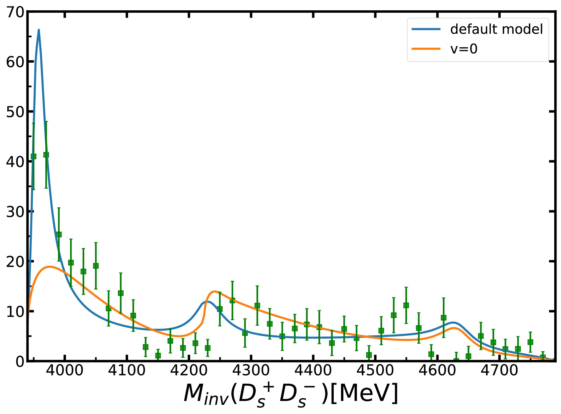

Figure 3.  (color online) Comparison of different models. The blue line in the figure is for the default model, whereas the orange line is for the model that turns off the couple-channel effect.

We analyze the observations of the LHCb Collaboration on the decay process $ B^+\to D_s^+D_s^-K^+ $. Note that when calculating the total amplitude, we refer to the work of the LHCb Collaboration and introduce the Breit-Weigner effect of the resonance state $ \psi(4260) $, but the peak value of $ \psi(4260) $ is slightly earlier than the jump position in the data of the invariant mass spectrum of $ D_s^+D_s^- $, and this position is very close to the threshold of $ D\bar{D} $. Therefore, we can reasonably expect that building a new model based on our current model and adding $ D\bar{D} $ this coupled-channel will be useful in explaining the jump in the invariant mass spectrum of $ D_s^+D_s^- $. Our default model fits the $ M_{D_s^+D_s^-} $, $ M_{D_s^+K^+} $, and $ M_{D_s^-K^+} $ of these three different invariant mass distributions simultaneously, and the final fitting quality is $ \chi^2/ndf\simeq1.31 $.

Without adding resonance states directly, we search the poles of $ X(3960) $ and $ X_0(4140) $ using the coupled-channel model and finally determine the positions of $ X(3960) $ and $ X_0(4140) $. From this, we suggest that $ X(3960) $ may be a resonance state and $ X_0(4140) $ may be a virtual state. The determination of the pole positions is meaningful, which provides information for the research on $ X(3960) $ and $ X_0(4140) $ and lays a certain foundation for the study of their properties in the future. By turning off the coupled-channel effect and fitting the data again, we find that the overall fitting quality does not change sigificantly. However, the final fitting result shows that the influence is relatively large at the position of $ X(3960) $, and almost all the changes of $ \chi^2 $ result from the $ X(3960) $ peak. Therefore, we suggest that the pure kinematic effect is insufficient to form the $ X(3960) $ peak structure. This conclusion provides certain reference value for future research.