Schwarzschild black hole surrounded by a cloud of strings in the background of perfect fluid dark matter

The prediction of black holes, one of the most profound and enigmatic outcomes of Albert Einstein’s General Theory of Relativity, has fascinated scientists for decades. This theoretical concept became an observational reality with the groundbreaking work of the Laser Interferometer Gravitational Wave Observatory (LIGO) collaboration, which not only detected gravitational waves that confirm a key aspect of General Relativity [1] but also recorded the unprecedented merger of two black holes [2]. Further validating these predictions, the Event Horizon Telescope (EHT) collaboration captured the first-ever image of a black hole’s shadow in the galaxy Messier 87 (M87*) [3], and later, it imaged Sagittarius A*, the supermassive black hole at the center of the Milky Way [4]. These extraordinary discoveries by LIGO and EHT have revolutionized astrophysics, not only opening new frontiers in black hole research but also providing a foundation for detailed analyses of their fundamental properties.

One of the key features in black hole imagery is the shadow it casts [5]. This shadow appears as a two-dimensional dark area in the sky, formed by light rays bent around the black hole’s event horizon due to the extreme curvature of spacetime [6]. The size and shape of the shadow provide crucial information about the black hole's mass, spin, and surrounding spacetime geometry [7]. For instance, a Schwarzschild black hole (SBH), which is non-rotating and spherically symmetric, forms a perfectly circular shadow. In contrast, a Kerr black hole, characterized by its rotation, produces an asymmetric and elongated shadow due to the frame-dragging effect of its spin. The study of these shadow shapes has become a critical observational tool for understanding black hole properties, fueling a rapid increase in related research literature; examples of such studies can be found in [8−49].

The environment around a black hole, such as the presence of dark matter, can significantly affect the characteristics of its shadow. Studies have shown that when a black hole is surrounded by dark matter, the distribution of this matter can influence the shadow’s size and shape. For example, black holes with dark matter halos exhibit shadows that can either increase or decrease in size depending on the density and proximity of the dark matter to the black hole. If the dark matter is highly concentrated near the black hole, it could distort the spacetime and thus alter the shadow’s appearance, making it more detectable. In particular, the photon orbits (or paths light takes around the black hole) can be altered by the presence of dark matter, leading to variations in the shadow’s intensity and geometry compared to a vacuum SBH [50−56].

In string theory, the concept that fundamental particles are replaced by one-dimensional strings has led to new perspectives on black holes, particularly with the idea that a cloud of strings (CoS) could serve as a source of the gravitational field. Letelier first proposed this model, providing an exact solution for an SBH surrounded by a CoS [57]. Since then, further research has explored the impact of these string clouds on various black hole solutions [58−73]. For example, Toledo et al. [58] studied the thermodynamics of a Reissner–Nordström black hole surrounded by a quintessence matter field and CoS, while Costa et al. [59] focused on similar aspects for an SBH. Subsequently, Cárdenas et al. [60] explored the astrophysical implications of an SBH associated with a CoS and quintessence through standard general relativistic tests conducted in the solar system, revealing potential modifications to gravitational interactions and celestial dynamics. Additionally, the authors examined the motion of photons and test particles [62], as well as the shadow, photon sphere [63], and gravitational weak lensing [64] in an SBH influenced by quintessence and string clouds, highlighting their impact on black hole observations and behavior. In [66], Rodrigues et al. demonstrated that the Bardeen black hole becomes singular in the presence of a string cloud, while the Simpson–Visser solution remains regular. Soon after, it was found that the quasinormal modes of the Bardeen black hole are significantly affected by the presence of a string cloud [68], along with alterations to its thermodynamic properties and geometry [69]. Moreover, studies by Yang et al. [70] demonstrated that the string cloud parameter plays a crucial role in shaping the shadow of rotating black holes, influencing black hole mimicry and the behavior of quasinormal modes. Recently, in [72] and [73], the authors investigated the effects of quantum corrections raised by generalized and extended generalized uncertainty principles on the images and stability of black holes with a CoS, respectively.

However, the need to study dark matter remains critical, as it makes up approximately 27% of the universe's total energy density, yet its true nature continues to be one of the greatest unsolved mysteries in modern physics. Understanding dark matter is essential not only for explaining galaxy formation and large-scale cosmic structures but also for investigating its interaction with dark energy, which drives the accelerated expansion of the universe. In this context, the perfect fluid dark matter (PFDM) model offers an intriguing framework for exploring the role of dark matter, particularly in relation to black holes. Unlike standard particle-based models, the PFDM model treats dark matter as a continuous, non-viscous fluid governed by specific equations of state that shape its dynamics [74]. This model has been applied to scenarios where dark matter clusters around black holes [75], altering their observable properties. For instance, the PFDM model predicts modifications to black hole metrics, such as changes to the Kerr [76−78], Schwarzschild [79, 80], Reissner-Nordström [81], Bardeen [82], or Euler-Heisenberg [83, 84] solutions, potentially influencing geodesics [85−87], gravitational wave signals [88, 89], stability and phase transitions [90−92], lensing [93], accretion discs [94], shadows [95, 96], deflection angle [97], quasinormal modes [98], greybody factors [99], thermodynamics [100−102], and event horizon structures [103]. These deviations provide new insights into the nature and distribution of dark matter in galactic halos, offering a novel means to reconcile cosmological observations with black hole physics. As a result, the PFDM model presents a promising alternative to traditional dark matter theories, particularly in explaining phenomena at galactic and cosmological scales.

In a recent article [92], Sood et al. explored Letelier black holes in AdS spacetime surrounded by PFDM, revealing significant insights into phase transition phenomena, photon orbits, and critical behaviors. Motivated by these findings, we aim to extend the investigation to an SBH immersed in a CoS and PFDM, focusing specifically on the case without the influence of AdS spacetime. Our study examined the black hole’s thermodynamics, shadows, geodesics, and quasinormal modes, with the goal of understanding how the presence of PFDM and string clouds affects these fundamental properties. Through this exploration, we seek to uncover new insights into the interaction between dark matter, string structures, and black hole dynamics, offering a deeper understanding of their microphysical nature and potential astrophysical signatures.

The remainder of the manuscript is organized as follows: Section II provides an overview of the mathematical framework for the SBH in the presence of a CoS and PFDM. Section III discusses the black hole's thermodynamic properties, highlighting the effects of the string and PFDM parameters. Section IV explores the geodesic structure, followed by Section V, which examines the black hole’s shadow in the context of a CoS and PFDM. Section VI investigates the quasinormal modes of the system. Finally, the manuscript concludes with a summary of the key findings. It is important to note that throughout the manuscript, natural units are adopted, where $\hbar=k_{B}= G=c=1$.

In this section, we aim to derive the Schwarzschild solution for a spacetime surrounded by a CoS in the presence of PFDM. To achieve this, we consider the following action:

where g is the determinant of the metric tensor $ g^{\mu \nu} $ and R denotes the scalar curvature. Here, ${\cal{L}}^{\rm PFDM}$ represents the Lagrangian density for PFDM, and $S^{\rm CS}$ corresponds to the Nambu-Goto (NG) action, which describes string-like objects, as defined in [57, 66]:

In this action, $ {\cal{M}} $ denotes a dimensionless constant that characterizes the string. The parameters $ \lambda ^{0} $ and $ \lambda ^{1} $ are timelike and spacelike parameters, respectively, while γ represents the determinant of $ \gamma _{ab} $, which is the induced metric on a submanifold defined by

Using a spacetime bivector $ \Pi ^{\mu \nu }=\epsilon ^{ab}\dfrac{\partial x^{\mu }}{\partial \lambda ^{a}}\dfrac{\partial x^{\nu }}{\partial \lambda ^{b}} $, we can express the NG action as

where $ \epsilon ^{ab} $ is the Levi-Civita symbol, and $ \epsilon^{01}=-\epsilon ^{10}=1. $ We then vary the total action given in Eq. (1) with respect to the metric and obtain the field equations

In this formulation, the energy-momentum tensor for the CoS is expressed as

where the only non-vanishing component of the bivector $ \Pi ^{01}=-\Pi ^{10} $ is a function of the radial coordinate. This component is explicitly written as

leading to

where a is an integration constant associated with the strings, constrained within the range $ 0<a<1 $.

Meanwhile, the second tensor, which represents the energy-momentum tensor for the PFDM, is written in the conventional orthonormal reference frame as follows [104]:

Here, ρ denotes the energy density and is expressed in terms of the PFDM constant α as

and the remaining components correspond to the radial and angular pressures.

Now let us consider a spherically symmetric spacetime, characterized by the metric function $ f(r) $, which depends on the radial coordinate r and is given by the form

where $ m(r) $ is the mass function. Then, we employ the corresponding line element

in conjunction with Eqs. (6) and (9). Substituting these expressions, we find that the time component of Eq. (5) simplifies to

We then integrate Eq. (13) from r to $ \infty $, obtaining the metric function for the SBH in the presence of the CoS and PFDM as follows:

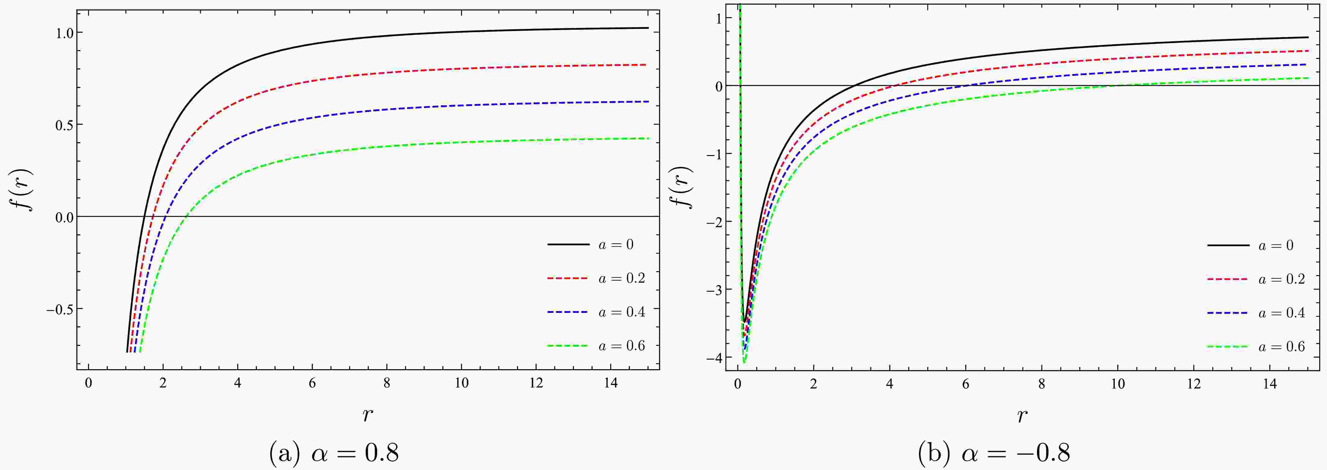
It should be noted that this metric function is the same as that given by Sood et al. in [92] in the absence of the AdS spacetime term. Moreover, for $ \alpha =0 $, the metric function, which we obtained in Eq. (14), reduces to that of the SBH with a CoS background [57]. In the case where $ a=0 $, the metric function describes the SBH immersed in PFDM [80]. In the scenario where both α and a are zero, the metric function reduces to the traditional metric function of the SBH.

To examine the impact of the CoS and PFDM on the black hole, we plot the metric function versus radius in Fig. 1. We consider both positive and negative values of α in the remainder of our analysis to explore the full range of possible effects on black hole properties.

Figure 1.  (color online) Effect of the CoS on the $ f(r)-r $ diagrams of the SBH surrounded by PFDM.

In both scenarios, increasing the CoS parameter causes a downward shift in the metric function, thereby influencing the horizon's location. For $ \alpha = 0.8 $, as the CoS parameter increases, the metric function reaches positive values at progressively larger radial distances, effectively moving the horizon outward. In contrast, a distinct structural configuration emerges in the scenario with $ \alpha = -0.8 $. As shown in Fig. 1(b), the metric function displays two distinct horizons: event horizon $ r_{H} $ and inner Cauchy horizon $ r_{C} $, in contrast to the single horizon observed in Fig. 1(a). This result indicates that the PFDM parameter has a substantial impact on spacetime curvature, and consequently, on the black hole’s thermal properties, particularly in relation to its stability. Finally, as r increases, the metric function approaches a constant value in both cases, with the influences of a and α diminishing at larger radii.

Compared with the existing literature, we observe similar results. For instance, Al-Badawi et al. [72], who investigated GUP-corrected black holes in the presence of a CoS, found that increasing the CoS parameter values leads to a larger horizon radius, a trend that also holds in our study for both positive and negative PFDM scenarios.

In this section, we discuss the thermodynamic characteristics of the black hole modeled by Eq. (14). We start by calculating the mass of the black hole using the condition $ f(r_H) = 0 $, where $ r_H $ is the event horizon radius. This leads to the following expression for the black hole mass:

For $ a=0 $, Eq. (15) simplifies to

which describes the mass of the SBH surrounded by PFDM [80]. Instead, if one sets $ \alpha=0 $, then Eq. (15) reduces to the mass of the SBH in the presence of CoS [57]:

Further, for $ \alpha=a=0 $, we retrieve the mass of a standard SBH.

The temperature associated with a black hole, referred to as the Hawking temperature, is directly proportional to its surface gravity κ, with the relationship expressed by the equation $ T = \dfrac{\kappa}{2\pi} $, where the surface gravity κ is defined as

Using Eqs. (14) and (18), we derive a relationship between the black hole's temperature and horizon radius in the following form:

We note that the Hawking temperature reduces to $ T=\dfrac{1-a}{4\pi r_{H}} $ when $ \alpha =0 $ and to $ T=\dfrac{1}{4\pi r_{H}}\left( 1+\dfrac{\alpha }{r_{H}}\right) $ when $ a=0 $, as shown in earlier works [57, 80], while in the absence of both SoC and PFDM, Eq. (19) yields the usual form of $ T=\dfrac{1}{4\pi r_{H}} $.

In Fig. 2, we plot the Hawking temperature of the SBH immersed in PFDM and surrounded by a CoS for two distinct scenarios and various parameter values. In a scenario with a positive PFDM parameter, the temperature indicates that the SBH is cooling down monotonically by the Hawking radiation as its size increases. Comparison between Fig. 2(a) and Fig. 2(b) reveals that for negative PFDM parameters, the divergence observed with positive PFDM parameters disappears. Moreover, during the evaporation process, the Hawking temperature initially increases, reaching a maximum value of

Figure 2.  (color online) Temperature versus horizon radius for different values of a in two PFDM scenarios.

at the critical horizon radius

before rapidly dropping to zero at the black hole's minimum size,

Additionally, as the value of the CoS parameter increases, the overall temperature decreases for a given horizon radius. This effect is consistent across both figures, suggesting that a stronger CoS reduces the Hawking temperature. The temperature tends to converge for large horizon radii, indicating that the effects of the CoS and PFDM become less significant for relatively larger black holes.

We then derive the SBH entropy function by utilizing the formula

Using Eqs. (15) and (19), the black hole entropy is expressed in its conventional form as [80, 92]

We note that the CoS and PFDM do not explicitly affect the entropy, which remains linearly proportional to the area. It is worth noting that the CoS and PFDM parameters do have a direct impact on the black hole and its entropy through the event horizon.

Next, we investigate the thermodynamic stability by utilizing the heat capacity, which is defined as

By substituting Eqs. (19) and (24) into Eq. (25), we obtain

It is worth noting that, unlike the entropy function, the heat capacity explicitly depends on both the string cloud and PFDM coefficients. In the absence of these parameters, specifically in the limit $ a \rightarrow 0 $, Eq. (26) reduces to

as given in [80]. Notably, in the absence of the PFDM parameter $ \alpha=0 $, Eq. (26) gives the standard form

which indicates that the presence of the string cloud does not directly influence the specific heat. For further analysis, Fig. 3 plots the heat capacity for a Schwarzschild black hole surrounded by the CoS and PFDM.

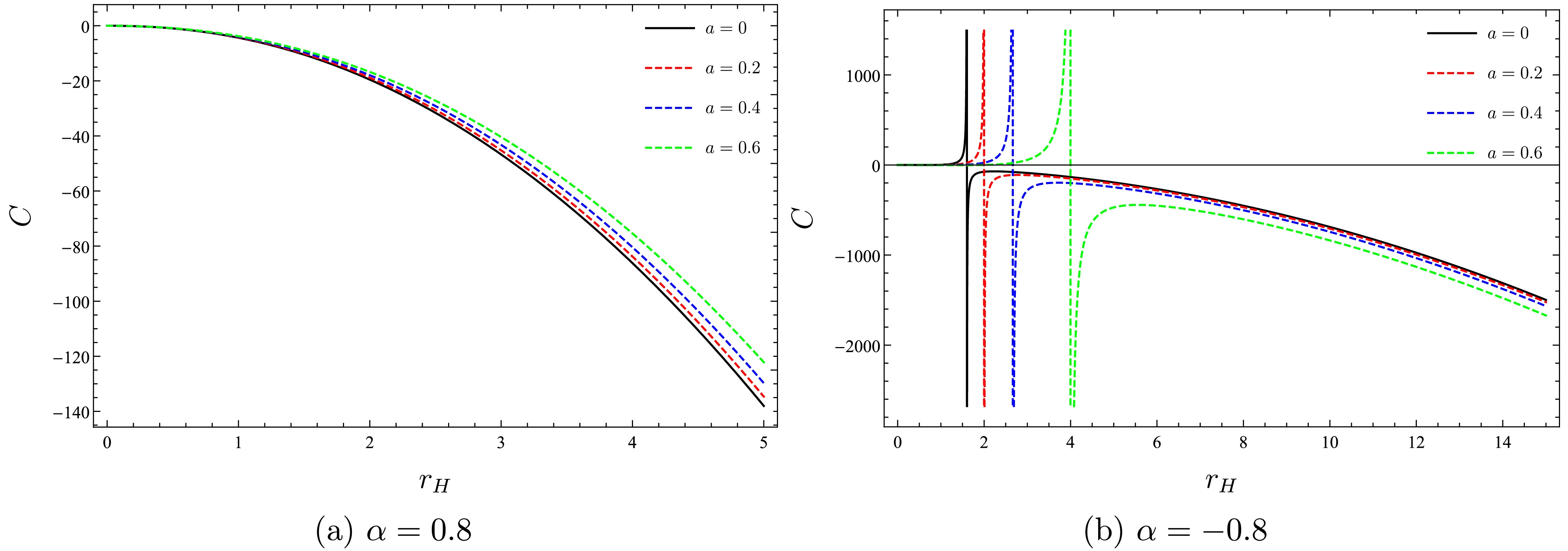
Figure 3.  (color online) Heat capacity versus horizon radius for different values of a in two PFDM scenarios.

Figure 3(a) illustrates the behavior of heat capacity with the positive PFDM parameter. The results show that the heat capacity is consistently negative, which signifies the thermodynamic instability of the black hole. Notably, the curves for varying values of a are distinct, particularly for larger values of $ r_{H} $. In contrast, Fig. 3(b) depicts the heat capacity with a negative PFDM parameter, where we observe that the heat capacity reaches zero at $r_{H}=r_{\min}$, marking the minimum size at which the black hole ceases to radiate. The stable black hole is characterized by a positive heat capacity within the range $ r_{\min}<r_{H}<r_{\rm crt} $, indicative of a smaller black hole. Conversely, for $ r_{H}>r_{\rm crt} $, the system becomes unstable, exhibiting a negative heat capacity associated with a larger, more massive black hole. Additionally, the stable range $ r_{\min}<r_{H}<r_{\rm crt} $, where the heat capacity remains positive, expands as a increases. This observation suggests that smaller values of a result in a quicker cessation of radiation and evaporation for the black hole.

In comparison to existing works, such as that by Chaudhary et al. [73], which demonstrated that the CoS induces critical regions where black holes transition between stability and instability under EGUP corrections, our findings further highlight that the CoS, in conjunction with PFDM, significantly modifies the thermodynamic properties and stability thresholds of black holes.

To further examine the phase transition and thermodynamic stability, we now focus on the Gibbs free energy, defined as

By substituting Eqs. (16), (19), and (24) into Eq. (29), we get

In Fig. 4, we illustrate the variation of the free energy with respect to $ r_{H} $.

Figure 4.  (color online) Gibbs free energy function versus event horizon with different values of a for $ \alpha=-0.8 $.

We observe that the Gibbs free energy reaches a minimum at

and the value of this horizon shifts with a decrease in the CoS and/or PFDM parameter, corresponding to a stable region.

The geodesic equations, along with their corresponding constraint equations, as given in [105], are as follows:

where $ \eta =0 $ for null geodesics and $ \eta =1 $ for timelike geodesics. In this context, the dot indicates differentiation with respect to the affine parameter s, while x refers to the spacetime coordinates. For a given spherically symmetric black hole metric, the geodesic equations take the following form:

Here, the prime symbol is used to indicate differentiation with respect to the spatial coordinate r. After some algebraic manipulation, the constraints for null and timelike geodesics is found to be

These equations, along with Eqs. (34)−(38), can be utilized to analyze the behavior of geodesic equations on the equatorial plane, as is done for the SBH in the absence of PFDM and CoS. By setting $ \theta =\pi /2 $, which implies $ \dot{\theta}=\ddot{\theta}=0 $, the geodesic equations simplify, and one can integrate Eqs. (34) and (37), resulting in

Here, the integration constants E and L refer to conserved quantities of the test particles: E corresponds to the total energy, and L represents the angular momentum. Substituting Eqs. (39) and (40) into the constraint equation given in Eq. (38), the energy conservation equation for null geodesics becomes

where the effective potential is found to be

From Eq. (42), one can analyze both time-like and null geodesics for different values of PFDM and CoS.

The effective potential plays a critical role in analyzing the trajectories of test particles, enabling us to describe their trajectories without explicitly relying on the equations of motion. The extrema of the effective potential delineates stable and unstable circular orbits, with maximum values indicating unstable orbits and minimum values indicating stable ones. For timelike trajectories, where $ \eta =1 $, the effective potential for particles can be expressed as

Here, the first term refers to the Newtonian gravitational potential, while the second term accounts for a repulsive centrifugal potential. The third term introduces a relativistic correction arising from general relativity, with a magnitude proportional to a specific factor $ 1/r^{3} $. Lastly, the fourth and fifth terms stem from the presence of a CoS and PFDM, respectively.

We note that the effective potential is governed by several parameters, including the mass M, angular momentum L, CoS parameter a, and PFDM parameter α. By fixing two of these parameters, $ M=1$ and $ L=10 $, in Fig. 5, we present the effective potential curves for different values of α in two distinct cases: $ a=0.2$ and $ 0.4 $.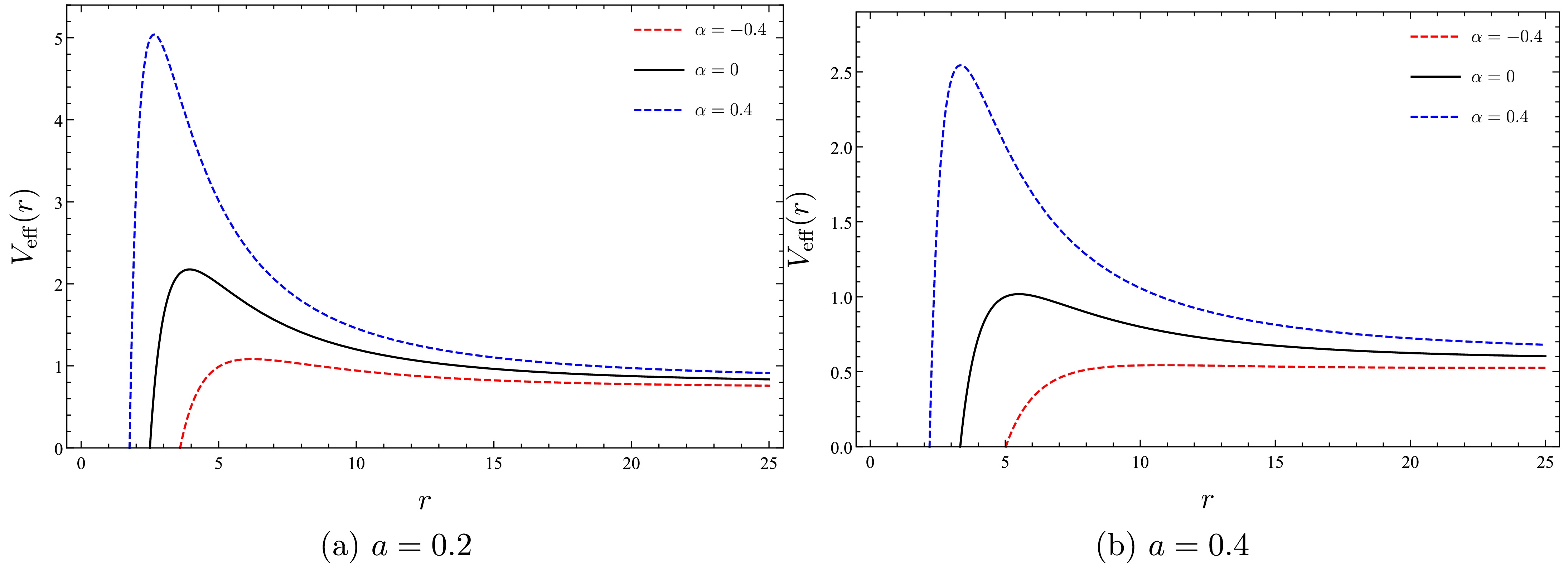

Figure 5.  (color online) Behaviors of timelike geodesic effective potential with different values of parameter PFDM α, with $ L=10 $.

The above figure demonstrates that as α increases, the maximum peak of the effective potential rises. Moreover, for a fixed value of α, increasing the string cloud parameter a causes the overall height of the effective potential to decrease, with the curves shifting downward.

Now, let us focus on Eq. (41), which describes the relationship between the energy and effective potential, where these energy levels govern the motion of particles. We then consider three specific energy levels: $ E_{1},E_{2} $, and $ E_{c}=E, $ with $ E_{c}^{2}-V_{\rm{eff}}\left( r\right)=0 $ as shown in Fig. 6.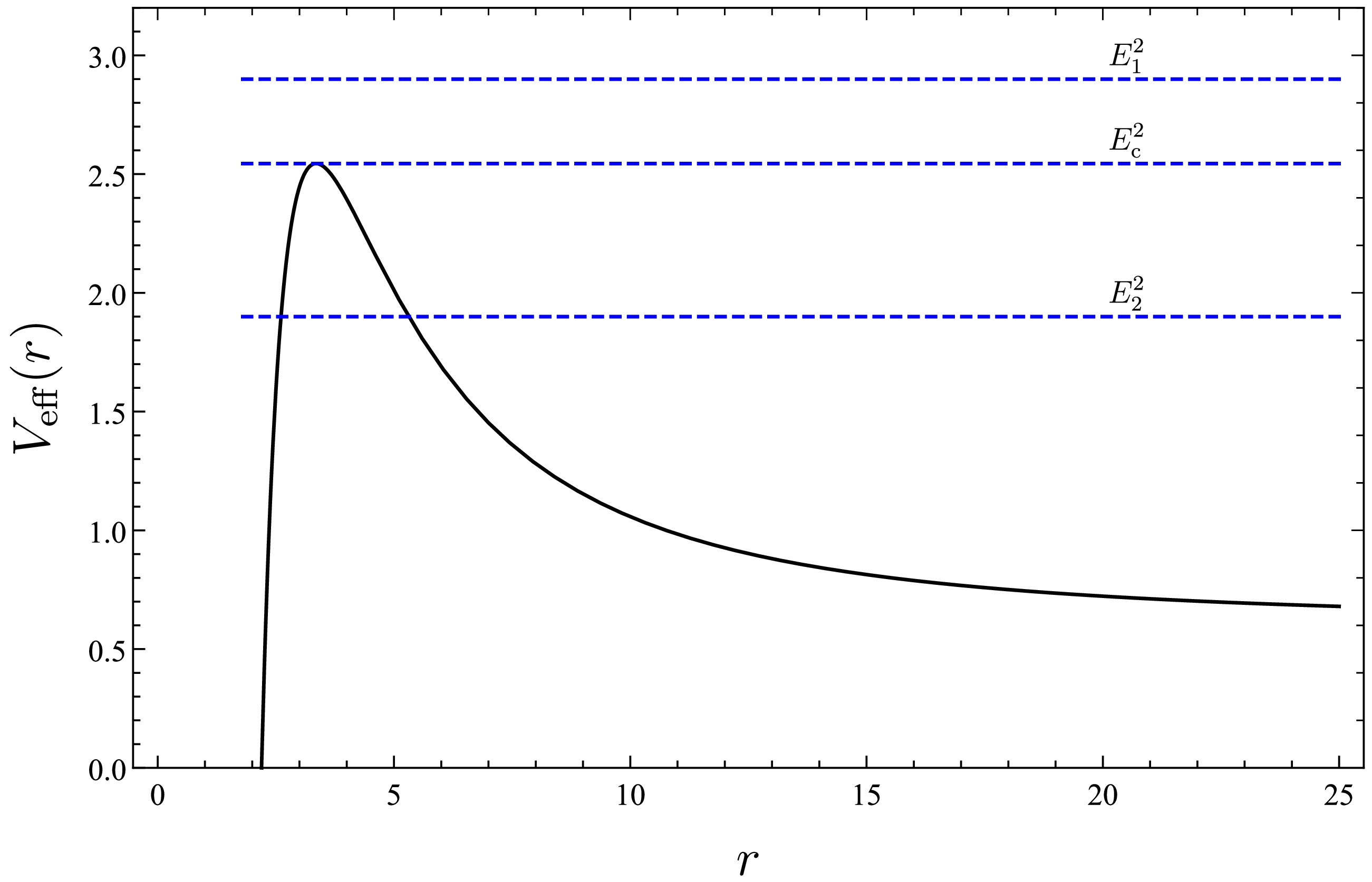

Figure 6.  (color online) Effective potential for a unit mass of black hole, with an angular momentum value of $ L=10 $.

For these distinct constant energy values, the permitted orbits are as follows:

• If $ E<E_{c} $, the particles can travel from infinity to a minimum distance before returning to infinity. In this scenario, the particles undergo only deflection. The other permitted orbits correspond to photons moving on the opposite side of the potential barrier, ultimately leading them toward the singularity.

• If $ E=E_{c} $ the particles can orbit in an unstable circular trajectory and the orbit radius is influenced by the parameters $ a, $ $ M, $ $ L, $ and α.

• If $ E>E_{c} $, the particles approach from infinity and move partially around the central mass from a very large distance before plunging into the singularity. Thus, the trajectory of the particles does not constitute a stable orbit around the black hole; instead, it ultimately leads to their absorption by the black hole. We demonstrate this scenario in Fig. 7.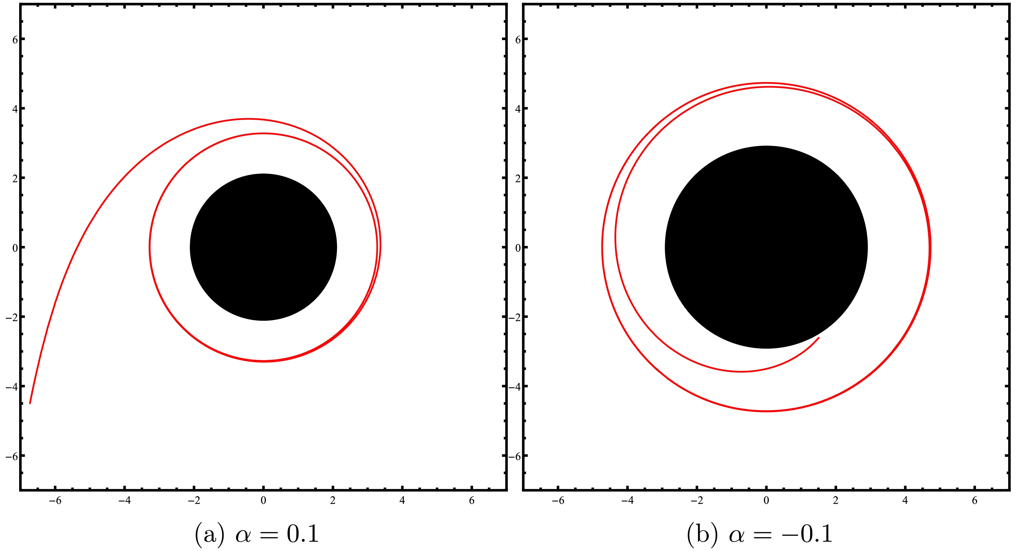

Figure 7.  (color online) Plots of the timelike unstable circular orbits for $ L=10 $, $ M=1 $, and $ a=0.2 $.

We will now examine circular orbits and their stability conditions to understand the influence of PFDM and CoS on this type of orbit. A circular orbit is established when the following two conditions are satisfied:

and

By solving the above equations, we can obtain the radii of circular orbits for specified values of angular momentum

and total energy

In astrophysics, the innermost stable circular orbit (ISCO) plays a crucial role in characterizing the dynamics of a test body in the gravitational field of a compact object. This orbit is described by the convergence of the maximum and minimum points of the effective potential. To accurately determine the ISCO's radius, an additional condition is required: the second derivative of the effective potential with respect to the radius must be zero, i.e.,

Now, by employing Eq. (46) along with this condition, we obtain

Before concluding this subsection, we conduct a numerical investigation of the parameters $ r_{\rm{ISCO}} $, $ L_{\rm{ISCO}} $, and $ E_{\rm{ISCO}} $. The results of our calculations for various scenarios are summarized in Table 1 for convenient reference and comparison.

a	$ \alpha =0.1 $				$ \alpha =0.3 $
	$ r_{\rm{ISCO}} $	$ L_{\rm{ISCO}} $	$ E_{\rm{ISCO}} $		$ r_{\rm{ISCO}} $	$ L_{\rm{ISCO}} $	$ E_{\rm{ISCO}} $
$ 0 $	5.22562	2.89896	0.951969		4.84986	2.41591	0.973802
$ 0.2 $	6.45311	3.57809	0.851569		5.85946	2.89992	0.872041
$ 0.4 $	8.46861	4.69245	0.737597		7.46782	3.66196	0.756472
$ 0.6 $	12.4167	6.87326	0.602386		10.4855	5.06536	0.619279
	$ \alpha =-0.1 $				$ \alpha =-0.3 $
$ 0 $	6.87751	4.0847	0.936026		7.7918	4.83513	0.925127
$ 0.2 $	8.68426	5.15634	0.837268		10.0209	6.2065	0.827892
$ 0.4 $	11.7291	6.96182	0.725161		13.8429	8.5538	0.717428
$ 0.6 $	17.9108	10.6259	0.592165		21.7779	13.4167	0.586256

Table 1.  Numerical values of the ISCO parameters $ r_{\rm{ISCO}} $, $ L_{\rm{ISCO}} $, and $ E_{\rm{ISCO}} $ for test particles, tabulated for various possible scenarios.

For lightlike particles, where $ \eta =0 $, the effective potential reduces to

Figure 8 illustrates the effective potential for $ a=0.4 $ and $ 0.2 $ with various PFDM values.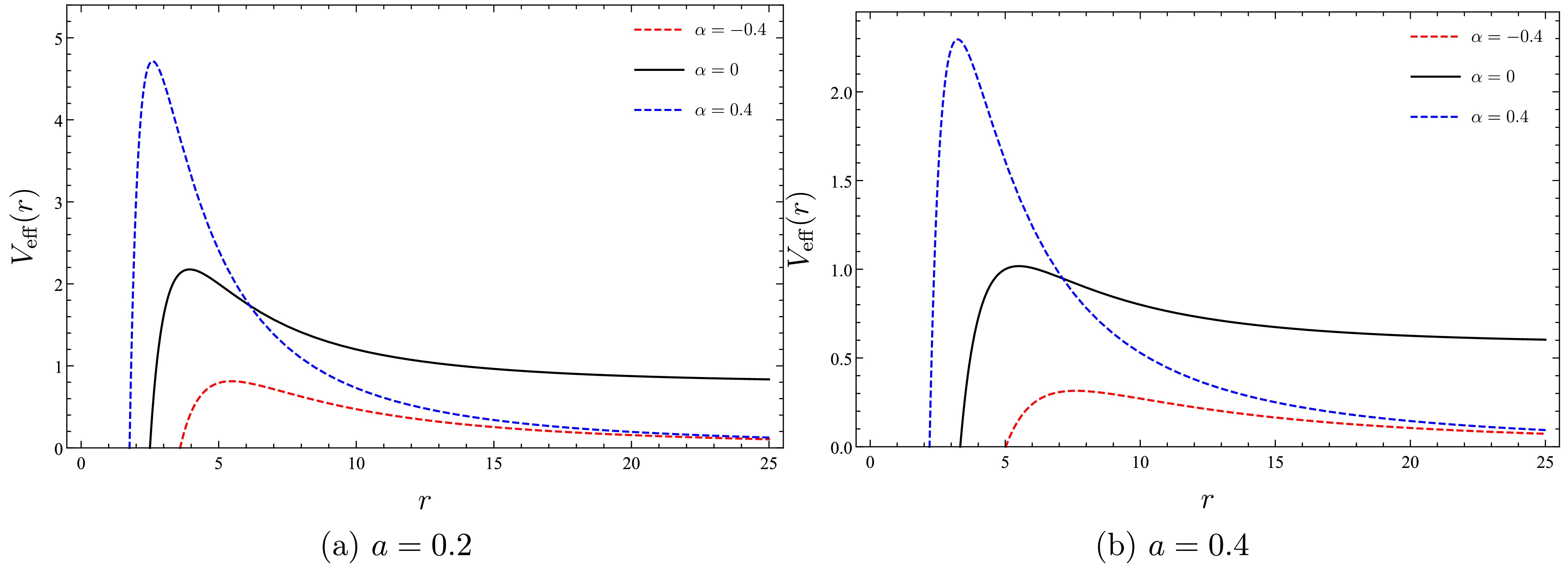

Figure 8.  (color online) Effective potential for null geodesics with different values of the PFDM parameter for $ L=10 $.

The graph shows the effective potential rising to a peak at the photon sphere radius, denoted as $ r_{\rm{ph}} $, before declining to zero. The behavior of lightlike geodesics is notably simpler than that of timelike geodesics. Each curve for the effective potential exhibits a single energy maximum, which characterizes an unstable circular orbit. As the PFDM increases, the maximum value of the effective potential also increases. Conversely, when the CoS parameter decreases, the peak value of the effective potential rises.

We now examine the radius of the photon sphere $ r_{\rm{ph}} $ and the associated instability condition to understand how the presence of PFDM and a string cloud affect it. For this purpose, we consider the scenario of circular orbits, $ \dot{r}=0 $, where the corresponding effective potential must satisfy the following conditions:

Additionally, the condition for instability requires that

Using the first condition given in Eq. (51), we obtain

where ξ is the impact parameter, defined as $ \xi=\dfrac{L}{E} $. Using the second condition given in Eq. (52), we find that

In this case, finding an exact analytical solution to Eq. (55) is not feasible. Therefore, we resort to numerical methods to solve it. The introduction of PFDM and the string cloud introduces two new parameters into Eq. (55). We will explore various values for these parameters and employ numerical techniques to determine the radius of the photon sphere. Subsequently, we will compute the corresponding impact parameter ξ and present the results in Table 2.

a	$ \alpha =0.1 $			$ \alpha =0.5 $			$ \alpha =0.9 $
	$ r_{\rm{ph}} $	ξ		$ r_{\rm{ph}} $	ξ		$ r_{\rm{ph}} $	ξ
$ 0 $	2.56341	4.35581		2.15448	3.36190		2.22692	3.25507
$ 0.2 $	3.16475	6.01096		2.53910	4.40464		2.55304	4.11901
$ 0.4 $	4.15180	9.10280		3.12567	6.21022		3.02350	5.52730
$ 0.6 $	6.08438	16.3306		4.15484	9.97632		3.78084	8.19831
$ 0.8 $	11.6797	44.2970		6.58355	21.7074		5.29200	15.0674
	$ \alpha =-0.1 $			$ \alpha =-0.5 $			$ \alpha =-0.9 $
$ 0 $	3.48255	6.12047		4.37716	8.05550		4.81372	9.24671
$ 0.2 $	4.3969	8.63824		5.72275	11.7418		6.53234	13.9036
$ 0.4 $	5.93764	13.4673		8.05812	19.0293		9.56867	23.3003
$ 0.6 $	9.06513	25.1755		12.9812	37.3966		13.1115	51.9985
$ 0.8 $	18.6722	73.3053		28.9732	117.392		38.0181	156.816

Table 2.  Photon sphere radius and impact parameter for different values of PFDM and CoS with $ M=1 $.

Let us examine a light ray emitted by a stationary observer located at $ r_{\rm{O}} $, traveling into the past. The angle Θ between such a light ray and the radial direction is given by

Within this framework, the angular radius of the black hole shadow can be determined by taking the limit $ R\rightarrow r_{\rm{ph}} $ in Eq. (56):

When $ r_{\rm{O}}=r_{\rm{ph}} $, $ \Theta _{\rm{S}}=\pi /2 $, indicating that the shadow covers exactly half of the observer's sky. For a static observer located at a large distance, $ r_{\rm{O}}\rightarrow \infty $, the shadow radius of the black hole is found to be

With the black hole mass fixed at $ M=1 $, the shadow radii are illustrated in Fig. 9.

Figure 9.  (color online) Black hole shadow radius as a function of CoS for various PFDM parameters.

Using the equation above, we analyze the constraints on the parameter a based on the EHT data, as outlined in Table 3. To simplify the calculation, we use the metric of the SBH surrounded by a CoS in the absence of PFDM. In this scenario, the radii of the photon sphere and black hole shadow are respectively given by

	Mass/${M}_{\odot }$	Angular diameter/$ \mu {\rm{as}} $	Distance/kpc
Sgr. A$ ^{\ast } $	$ \left( 4.13\pm 0.013\right) \times 10^{6} $	$ 48.7\pm 7 $	$ 8.277\pm 0.033 $

Table 3.  Observational measurements of Sgr. A$ ^{\ast } $ black hole.

It is worth noting that our results indicate an inverse proportionality between the photon sphere radius and $ (1-a) $, a behavior also observed in the literature. In particular, in [72], Al-Badawi et al. demonstrated that both the photon sphere radius and impact factor, influenced by the presence of the CoS, exhibit the same inverse scaling with $ (1-a) $.

Then, we follow the bounds provided in [106]. For Sgr A$ ^{\ast } $, the permitted range is

Our results are presented in Fig. 10, which includes the confidence interval.

Figure 10.  (color online) Shadow radius $ \dfrac{R_{\rm{S}}}{M} $ of the SBH surrounded by CoS as a function of the string parameter.

While the overall shape of the curve remains consistent because of Eq. (60), we identify distinct upper bounds for a, as presented in Table 4.

	1σ upper	1σ lower
Sgr. A$ ^{\ast } $	$ 0.003 $	$ 0 $

Table 4.  Values of a based on the constraints imposed by the EHT data on the shadow radius.

The investigation of black hole quasinormal modes (QNMs) is long-established and thoroughly studied. The distinct frequencies of QNMs provide insights into the black hole's characteristics as well as the types of radiative emissions it can produce. Originally, these frequencies were computed using purely numerical methods. This involved selecting a complex frequency, solving the corresponding differential equation through numerical integration, and then verifying if the solution met the necessary boundary conditions. To the best of our knowledge, researchers have developed a variety of methods to study QNMs of black holes. These approaches include numerical Integration Methods [107], WKB Approximation [108−112], Leaver's Continued Fraction Method [113], Pöschl-Teller Potential Approximation [114], Asymptotic Iteration Method [115], and Time-domain Integration [116]. Additionally, it has been shown that the characteristics of QNMs can be related to the properties of photons trapped in unstable circular orbits around black holes [117−119]. In this section, we derive QNMs using two methods: the sixth-order WKB approximation and shadow radius method.

In curved spacetime, the dynamics of a massless scalar field are governed by the following equation:

To solve this, we adopt the ansatz

where ω represents frequency, $ \ell $ is the angular quantum number, and $ Y_{{\ell},\mu }\left( \theta ,\varphi\right) $ are the spherical harmonics. Substituting this decomposition into Eq. (62) transforms it into a Schrödinger-like equation:

where the tortoise coordinate $ r^{\ast } $ is related to r via ${\rm d}r^{\ast }=\dfrac{{\rm d}r}{f\left( r\right) }$. The effective potential $ {\cal{V}}\left( r\right) $ is given by

To solve Eq. (64), it is essential to impose appropriate boundary conditions. In this context, the physically acceptable solutions are those that represent purely ingoing waves near the black hole horizon, expressed as

Next, utilizing the WKB approximation, we compute the QNM frequencies using the following relation:

where $ V_{0} $ corresponds to the height of the effective potential, and $ V_{0}^{\prime \prime} $ denotes the second derivative of the potential with respect to the tortoise coordinate, evaluated at its maximum $ r_{0}^{\ast } $. The term $ \Lambda _{i} $ accounts for corrections from higher-order terms in the WKB approximation, while $n=0,1,2,\cdots$, is the overtone number.

Now, we calculate the QNM frequencies of the SBH by applying the 6th-order WKB approximation method for different angular quantum numbers $ \ell $ and overtone numbers n in the context of a massless scalar field. These frequencies are separated into real and imaginary components, where the real part refers to the oscillation frequency and the imaginary part corresponds to the decay rate. We tabulate the QNMs in Table 5.

$ {\ell} $	n	$ \alpha =0.3 $			$ \alpha =0.6 $
		$ \omega _{\rm{WKB}}(a=0.2) $	$ \omega _{\rm{WKB}}(a=0.5) $		$ \omega _{\rm{WKB}}(a=0.2) $	$ \omega _{\rm{WKB}}(a=0.5) $
1	0	0.306997–i 0.101910	0.162166–i 0.0436177		0.353318–i 0.128573	0.202572–i 0.060770
2	0	0.510563–i 0.100880	0.273616–i 0.0433136		0.586499–i 0.126928	0.341274–i 0.0602066
	1	0.488732–i 0.308314	0.265861–i 0.131531		0.555395–i 0.389586	0.328738–i 0.183452
3	0	0.714401–i 0.100589	0.384350–i 0.0432315		0.820241–i 0.126460	0.479200–i 0.0600535
	1	0.698288–i 0.304695	0.378717–i 0.130505		0.797165–i 0.383912	0.470059–i 0.181602
	2	0.668314–i 0.517244	0.367940–i 0.220160		0.754681–i 0.654423	0.452703–i 0.307391
4	0	0.918318–i 0.100469	0.494845–i 0.0431980		1.05415–i 0.126265	0.616865–i 0.0599908
	1	0.905622–i 0.303186	0.490435–i 0.130084		1.03594–i 0.381548	0.609698–i 0.180844
	2	0.881281–i 0.511134	0.481841–i 0.218425		1.00120–i 0.644934	0.595790–i 0.304287
	3	0.847393–i 0.727322	0.469526–i 0.309120		0.953375–i 0.921010	0.576018–i 0.431912

Table 5.  QNMs of the SBH surrounded by PFDM and CoS, calculated using the 6th-order WKB approximation method.

We observe that the imaginary components of all frequencies are negative, confirming the stability of the black hole. This also indicates the damping behavior of the oscillations, which is tied to the dynamical evolution of the QNMs.

Figure 11 illustrates the variation of the QNM frequencies of the SBH as a function of the overtone numbers for different values of the CoS parameter.

Figure 11.  (color online) QNMs of black holes in scalar field for the state $ \ell=7 $, $ \alpha=0.5 $, and $ M=1 $.

It is clear that for a fixed n, both $ \omega_{\rm{R}} $ and $ \omega_{\rm{I}} $ decrease as a increases. This suggests that a reduction in a results in an increase in the oscillation frequency and a faster decay rate. This result is consistent with the findings presented by Al-Badawi et al. in Table 2 of [72].

Next, by setting $ a=0.4 $, we examine the impact of PFDM on the QNMs, as depicted in Fig. 12.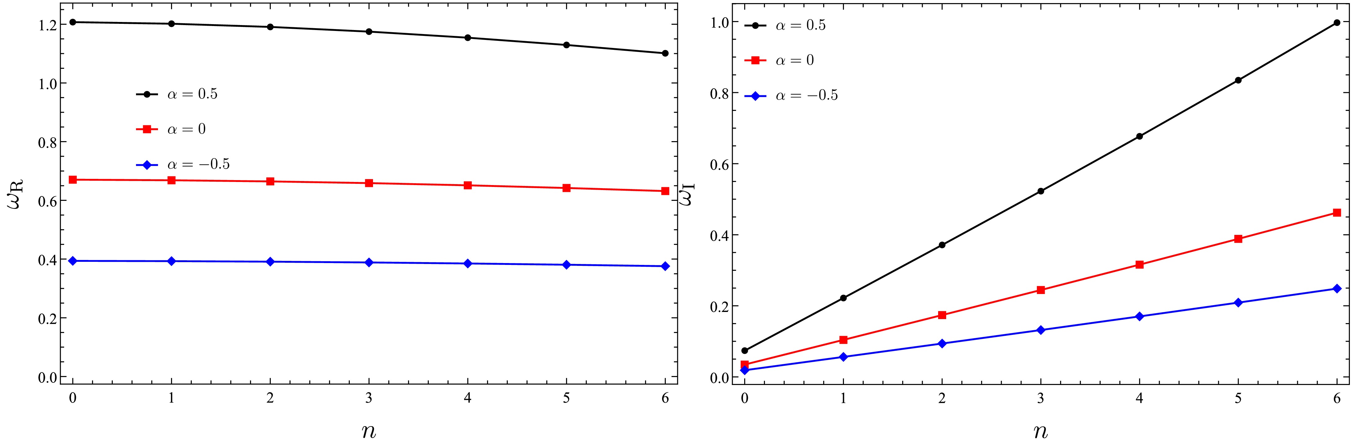

Figure 12.  (color online) QNMs of the SBH in the scalar field for the state $ \ell=7 $, $ a=0.4 $, and $ M=1 $.

It is apparent that for a fixed overtone number, both components of the frequencies, $ \omega_{\rm{R}} $ and $ \omega_{\rm{I}} $, increase with increasing PFDM parameter. This implies that a higher α enhances the oscillation frequency and decreases the rate of decay.

Previous studies [117−119] have established that in the eikonal limit, the real component of QNMs is related to the angular velocity of the final circular null geodesic, whereas the imaginary component is linked to the Lyapunov exponent,

where

represents the angular velocity of the photon sphere located at the unstable orbit, and

denotes the Lyapunov exponent.

Now, we compute quasinormal frequencies for scalar field perturbations across different angular momentum, PFDM, and CoS parameter values, utilizing Eqs. (67) and (68). By comparing the quasinormal frequencies for various values of angular momentum, we tabulate the results in Tables 6, 7, 8, and 9.

$ \ell $	$ \omega _{\rm{WKB}} $	$ \omega _{\rm{S}} $	$ \Delta _{\rm{R}} $%	$ \Delta _{\rm{I}} $%
$ 5 $	0.915073 – i 0.0766499	0.83182 – i 0.076572	10.009	0.10173
$ 7 $	1.24778 – i 0.0766139	1.1645 – i 0.076572	7.1516	5.4720 $ \times 10^{-2} $
$ 10 $	1.74685 – i 0.0765934	1.6636 – i 0.076572	5.0023	2.7948 $ \times 10^{-2} $
$ 15 $	2.57865 – i 0.0765818	2.4954 – i 0.076572	3.3361	1.2798 $ \times 10^{-2} $
$ 20 $	3.41046 – i 0.0765776	3.3273 – i 0.076572	2.4993	7.3134 $ \times 10^{-3} $
$ 30 $	5.07408 – i 0.0765745	4.9909 – i 0.076572	1.6666	3.2649 $ \times 10^{-3} $
$ 40 $	6.73771 – i 0.0765734	6.6545 – i 0.076572	1.2504	1.8283 $ \times 10^{-3} $
$ 50 $	8.40134 – i 0.0765729	8.3182 – i 0.076572	0.99950	1.1754 $ \times 10^{-3} $

Table 6.  QNMs calculated by 6th-order WKB approximation method and shadow radius, where $ a=0.2 $ and $ \alpha =0.1 $.

$ \ell $	$ \omega _{\rm{WKB}} $	$ \omega _{\rm{S}} $	$ \Delta _{\rm{R}} $%	$ \Delta _{\rm{I}} $%
$ 5 $	1.24912 – i 0.118982	1.1352 – i 0.118807	10.035	0.14730
$ 7 $	1.70307 – i 0.118901	1.5892 – i 0.118807	7.1652	7.9120 $ \times 10^{-2} $
$ 10 $	2.38408 – i 0.118855	2.2703 – i 0.118807	5.0103	4.0402 $ \times 10^{-2} $
$ 15 $	3.51917 – i 0.118829	3.4050 – i 0.118807	3.3530	1.8517 $ \times 10^{-2} $
$ 20 $	4.65430 – i 0.118820	4.5407 – i 0.118807	2.5018	1.0942 $ \times 10^{-2} $
$ 30 $	6.92459 – i 0.118813	6.8110 – i 0.118807	1.6677	5.0502 $ \times 10^{-3} $
$ 40 $	9.19490 – i 0.118810	9.0813 – i 0.118807	1.2509	2.5251 $ \times 10^{-3} $
$ 50 $	11.4652 – i 0.118809	11.352 – i 0.118807	0.99718	1.6834 $ \times 10^{-3} $

Table 7.  QNMs calculated by 6th-order WKB approximation method and shadow radius, where $ a=0.2 $ and $ \alpha =0.5 $.

$ \ell $	$ \omega _{\rm{WKB}} $	$ \omega _{\rm{S}} $	$ \Delta _{\rm{R}} $%	$ \Delta _{\rm{I}} $%
$ 5 $	0.636700 – i 0.0506996	0.578822 – i 0.0506555	9.9993	8.7059 $ \times 10^{-2} $
$ 7 $	0.868229 – i 0.0506792	0.810350 – i 0.0506555	7.1425	4.6787 $ \times 10^{-2} $
$ 10 $	1.21552 – i 0.0506676	1.15764 – i 0.0506555	4.9998	2.3887 $ \times 10^{-2} $
$ 15 $	1.79435 – i 0.0506610	1.73646 – i 0.0506555	3.3338	1.0858 $ \times 10^{-2} $
$ 20 $	2.37317 – i 0.0506587	2.31529 – i 0.0506555	2.4999	6.3172 $ \times 10^{-3} $
$ 30 $	3.53081 – i 0.0506569	3.47293 – i 0.0506555	1.6666	2.7638 $ \times 10^{-3} $
$ 40 $	4.68845 – i 0.0506563	4.63057 – i 0.0506555	1.2500	1.5793 $ \times 10^{-3} $
$ 50 $	5.84610 – i 0.0506560	5.78822 – i 0.0506555	0.99996	9.8706 $ \times 10^{-4} $

Table 8.  QNMs calculated by 6th-order WKB approximation method and shadow radius, where $ a=0.2 $ and $ \alpha =-0.1 $.

$ \ell $	$ \omega _{\rm{WKB}} $	$ \omega _{\rm{S}} $	$ \Delta _{\rm{R}} $%	$ \Delta _{\rm{I}} $%
$ 5 $	0.468360 – i 0.0348526	0.425829 – i 0.0348283	9.9878	6.9771 $ \times 10^{-2} $
$ 7 $	0.638706 – i 0.0348414	0.596161 – i 0.0348283	7.1365	3.7613 $ \times 10^{-2} $
$ 10 $	0.894216 – i 0.0348349	0.851658 – i 0.0348283	4.9971	1.8950 $ \times 10^{-2} $
$ 15 $	1.32006 – i 0.0348313	1.27749 – i 0.0348283	3.3323	8.6137 $ \times 10^{-3} $
$ 20 $	1.74589 – i 0.0348300	1.70332 – i 0.0348283	2.4992	4.8811 $ \times 10^{-3} $
$ 30 $	2.59756 – i 0.0348290	2.55497 – i 0.0348283	1.6669	2.0099 $ \times 10^{-3} $
$ 40 $	3.44922 – i 0.0348287	3.40663 – i 0.0348283	1.2502	1.1485 $ \times 10^{-3} $
$ 50 $	4.30088 – i 0.0348285	4.25829 – i 0.0348283	1.0002	5.7425 $ \times 10^{-4} $

Table 9.  QNMs calculated by 6th-order WKB approximation method and shadow radius, where $ a=0.2 $ and $ \alpha =-0.5 $.

We observe that as $ \ell $ increases, the differences in both the real and imaginary components of the frequency gradually diminish. This trend suggests that the eikonal limit method is highly accurate for large angular momentum values, producing results that closely align with the WKB approximation. This finding holds significant practical value, as the eikonal limit method is generally more straightforward for analytical computations. Furthermore, high-precision results provide reliable data for investigating the stability and oscillatory behavior of black holes and other compact objects.

Recent studies have indicated that the properties of black holes can be significantly influenced by their surroundings, including factors such as thermal stability, $ P-V $ criticality, quasinormal modes, shadow characteristics, and photon orbit radii. Inspired by these observations, we investigated the complex relationship between the SBH and its environment, characterized by PFDM and a CoS. Our analysis shows that the presence of the CoS and PFDM modifies the metric function, thereby impacting the black hole's horizon and mass. Furthermore, our examination of the Hawking temperature reveals distinct behaviors based on the parameters of PFDM: for positive parameters, the temperature consistently decreases, while for negative parameters, it initially rises to a maximum before cooling down, especially when the CoS parameters are relatively small. Additionally, our analysis of specific heat illustrates how the perfect fluid dark matter parameters affect the black hole's stability: with a positive parameter, the heat capacity remains consistently negative, indicating instability, whereas a negative parameter allows the heat capacity to reach zero at a certain point, marking the minimum size at which the black hole ceases to radiate. Notably, the Gibbs free energy provides insights into the stability of the black hole. Although the surroundings do not directly alter the black hole's entropy, which remains linearly proportional to the area, they influence the horizon, which, in turn, affects the entropy.

The geodesic structure and QNM analysis reveal how the CoS and PFDM significantly impact the black hole’s dynamics and observable characteristics. To do this, we first derived the effective potential, and then we investigated the stability of particle orbits, particularly altering the photon sphere and innermost stable circular orbit. We demonstrated that these changes have direct implications for the black hole's shadow radius. In other words, the study of null and timelike geodesics shows that the parameters of the CoS and PFDM strongly influence the trajectories of light and matter around the black hole. Furthermore, quasinormal mode analysis, using both the WKB approximation and shadow radius methods, indicated that the CoS and PFDM not only affect the oscillation frequencies but also the decay rates of the black hole’s perturbative modes. The real part of the QNM frequency is found to be linked to the angular velocity of the photon sphere, while the imaginary component is tied to the Lyapunov exponent, which governs the rate of mode decay. These results suggest that the presence of the CoS and PFDM can provide distinctive signatures in the black hole’s radiative and oscillatory behavior, potentially observable through gravitational wave detections. Such findings enhance our understanding of how exotic matter fields influence the stability, dynamics, and radiative properties of black holes, offering new pathways for testing theoretical models of dark matter and string clouds in astrophysical contexts.

Finally, it is important to emphasize that black holes should not be regarded as isolated entities. In nature, they constantly interact with their surroundings and are rarely unaffected by neighboring fields. Consequently, they are typically in a perturbed state due to the influence of other fields in their vicinity. The presence of PFDM and CoS around black holes offers valuable opportunities to test and expand gravity theories. PFDM modifies black hole thermodynamics and particle orbits, influencing key properties such as temperature, phase transitions, and gravitational lensing. These effects establish a bridge between the cosmological role of dark matter and its impact on black hole physics. Meanwhile, the CoS affects the geometry of spacetime and physical phenomena nearby. The mathematical structure of string theory has consistently demonstrated that it encompasses all the essential components for a quantum theory of gravity, including valuable insights into black hole entropy. However, string theory is not merely a theory of quantum gravity; it also incorporates particles and interactions, providing the tools necessary to address contemporary questions in cosmology. PFDM specifically addresses the coupling between dark matter and gravity, while the effects of CoS provide concrete tests of string theory-inspired modifications and potential signatures of quantum gravity. These predictions are particularly significant, as they can be tested using current and future observational facilities, such as LIGO/Virgo, the Event Horizon Telescope, and X-ray observatories.

We would like to express our sincere gratitude to the anonymous referee for their constructive suggestions and comments.