p-wave mesons emitting weak decays of bottom mesons

At present, large amounts of information is available on the decays of the heavy flavor hadrons, and more measurements are expected in future experiments. Worldwide, several groups at Fermi lab, Cornell, LHC-CERN, KEK, DESY, and Beijing Electron Collider, among others, have been working to provide wide knowledge of heavy flavor physics. One of the goals of heavy flavor hadron physics is also to elucidate the relationship among the particles of different generations [1].

Heavy, charm, and bottom mesons have revealed many channels for leptonic, semi-leptonic and hadronic decays. The b quark is especially interesting in this respect, as it has W-mediated transitions to both first-generation (u) and second-generation (c) quarks. The Standard Model (SM) is reasonably successful in explaining the leptonic and semileptonic decays, but the issue of weak hadronic decays is yet to be settled, and these decays have posed serious problems due to the strong interaction interference with the weak interactions responsible for these decays [2−7]. Initially, the weak hadronic decays of charm and bottom mesons were expected to have less interference due to the strong interactions, as their decay products carry large momenta. However, their measurements have revealed the contrary. The prominent reason being that experiments are producing data at the hadronic level, whereas the theory (SM) deals with quarks and leptons. Presently, the problem of Hadronization (formation of hadrons from quarks), being a low-energy phenomenon, cannot yet be resolved from first principles. In fact, understanding of the decays becomes more complicated as the produced hadrons in the weak hadronic decays can participate in the Final State Interactions (FSI) [8−19] caused by the strong interactions at the hadronic level. Therefore, analysis of weak hadronic decays requires phenomenological treatment, for which symmetry principles and quark models are often employed to explore the dynamics involved.

Even the weak interaction vertex itself is also affected through gluon-exchange among the quarks involved. At W-mass scale, hard gluons exchange effects are calculable using the perturbative QCD. Usually, factorization of weak matrix elements is performed in terms of certain form-factors and decay constants. Besides these high-energy gluon exchanges, there exist possible soft gluon exchanges around the W- vertex, which generate nonfactorizable contributions in the weak matrix elements [20−23]. The nonfactorizable terms may appear for several reasons, including soft gluon exchange and FSIrescattering effects [20−23]. The rescattering effects on the outgoing mesons have been studied in detail for bottom meson decays [24−25]. Besides that, flavor SU(3) symmetry and the Factorization Assisted Topological (FAT) approach have been employed for the study of such nonfactorizable contributions, as they have the advantage of absorbing various kinds of lump-sum contributions in terms of a few parameters, which can be fixed empirically [26, 27]. Extensive work has also been conducted to treat nonfactorizable contributions, such as the QCD factorization approach based on collinear factorization theorem [28] and the perturbative QCD factorization approach [29−30]. Unfortunately, it is not straightforward to calculate such terms, which are nonperturbative in nature and require empirical data to investigate their behaviour.

In the naïve factorization scheme, the nonfactorizable contribution for the decay amplitudes is completely ignored, and the two QCD coefficients a₁ and a₂ are fixed from the experimental data [31−33]. Initially, data on branching fractions of $ D \to \bar K\pi $ decays seemed to require $ {a_1} \approx {c_1} = 1.26,\;{a_2} \approx {c_2} = - 0.51, $ leading to destructive interference between color-favored (CF) and color-suppressed (CS) processes for $ {D^ + } \to {\bar K^0}{\pi ^ + }, $ thereby implying the $ {N_c} \to \infty $ limit [34]. However, later measurement of $ \bar B \to D\pi $ meson decays did not favor this result empirically, as these decays require $ {a_1} \approx 1.03, $ and $ {a_2} \approx 0.23, $ i.e., a positive value of $ {a_2} $, in sharp contrast to the expectations based on the large $ {N_c} $ limit, because the final state particles leave the interaction region very quickly, allowing little time for final state interactions, and soft-gluon exchange becomes less important [35]. Thus, B-meson decays, revealing constructive interference between CF and CS diagrams for $ {B^ - } \to {\pi ^ - }{D^0}, $ seem to favor $ {N_c} = 3 $(real value).

It has been found experimentally that two-body decays dominate the spectrum. Bottom meson decays to two s-wave mesons (pseudoscalar and vector mesons) have been studied reasonably well. Theoretical focus has also, so far, been on the s-wave meson ($ \bar B \to PP/PV $) emitting decays [1−24]. There exist four L=1 states: scalar $ ({J^{PC}} = {0^{ + + }}), $ axial-vectors $ ({J^{PC}} = {1^{ + \, + }} $and $ {1^{ + \, - }}) $, and tensor $ ({J^{PC}} = {2^{ + + }}) $ mesons. All these p-wave states and vector mesons decay to s-wave mesons through strong interactions, so these are called meson resonances. These states are generally produced either in scattering experiments or as decay products of heavy flavour mesons. Thus, we investigated the following decay modes involving one p-wave meson in the final state:

Branching fractions for some of the decay modes have been measured experimentally [1]. Kinematically, these decays are expected to be suppressed; however, the measured branching fractions of these modes are rather large. Therefore, it is desirable to study B- meson decays emitting p-wave mesons, which requires theoretical understanding.

Our group performed a thorough study of nonfactorizable contributions by using isospin analysis for $ D \to \bar K\pi /\bar K\rho /{\bar K^*}\pi $ decay modes and recognized a systematics for the ratio of nonfactorized reduced amplitudes. It is worth noting that this systematics was also found to be consistent with p-wave meson emitting decays of charm mesons: $D \to \bar K{a_1}/\pi {\bar K_1}/\pi {\bar K_{-1}}/\pi {\bar K_0}/\bar K{a_2}$ [22]. In our previous work [36], it was found that the nonfactorizable contributions in the respective 1/2 and 3/2 isospin reduced amplitudes for Cabibo-favored $ \bar B \to \pi D/\rho D/\pi {D^*} $ decay modes bear a universal ratio equal to $ \alpha $ within the experimental errors. Extension of this universality to $ \bar B \to {a_1}D/\pi {D_1}/\pi D'_1/\pi {D_2}/\pi {D_0} $ is hoped to yield useful predictions for their branching fractions. Therefore, in this paper, we extend our analysis to investigate nonfactorizable terms in the p-wave mesons emitting decays.

The remainder of this paper is organised as follow. In Section II, the weak Hamiltonian is expressed as a sum of two particle-generating factorizable and nonfactorizable contributions to the hadronic decays of B-mesons. In Section III, we introduce the methodology of our approach by analysing s-wave mesons emitting decays of bottom mesons. In Section IV, detailed analysis of p-wave meson emitting decays is presented. Summary and conclusions are given in the final section.

To study the two-body hadronic $ B - $decays, we consider the effective weak Hamiltonian [37]

where $ {V_{ud}} $ and $ {V_{cb}} $ are the Cabibbo–Kobayashi–Maskawa (CKM) matrix elements [1],

${\bar q_1}{q_2} = {\bar q_1}{\gamma _\mu }\left( {1 - {\gamma _5}} \right){q_2}$ denotes color singlet V−A Dirac current, and the QCD coefficients at the bottom mass scale are taken as [27, 38]

In the standard factorization scheme, the current operators in the weak Hamiltonian are expressed in terms of the fundamental quark fields. It is appropriate to have the Hamiltonian in a form such that one of these currents carries the same quantum numbers as one of the mesons emitted in the final state of bottom meson decays. Consequently, the hadronic matrix elements of the Hamiltonian operator $ {H_w} $ receive contribution from the operator itself and from its Fierz transformation. For instance, separating the factorizable and nonfactorizable parts of $(\bar du)(\bar cb)$using the Fierz identity [39] as

where ${\bar q_1}{\lambda ^a}\,{q_2} \equiv \,{\bar q_1} {\gamma _\mu }\,\left( {1 - {\gamma _5}\,} \right){\lambda ^a}{q_2}$ represents the color octet current, and performing similar treatment on the other operator $ (\bar cu)(\bar db), $ the weak Hamiltonian finally becomes

for the CF and CS processes, respectively, where

The subscript H in (4) and (5) indicates the change from quark current to hadron field operator. Matrix elements of the first terms in (4) and (5) lead to the factorizable contributions, and the second terms, involving the color octet currents, generate nonfactorizable contributions.

In this section, we describe our approach by analysing $ \bar B \to PP$ decay mode. The branching fraction for B-meson decay into two pseudoscalar mesons is related to its decay amplitude as follows:

where $ {\tau _B} $ denotes the lifetime of B-mesons measured to be [1]

and p is the magnitude of the 3-momentum of the final state particles in the rest frame of the parent B-meson:

Using the isospin framework, $ \bar B \to \pi D $ decay amplitudes are represented in terms of isospin reduced amplitudes ($ A_{1/2}^{\pi D} $, $ A_{3/2}^{\pi D} $) and the strong interaction phases ($ \delta _{1/2}^{\pi D},\,\; \delta _{3/2}^{\pi D} $) in respective Isospin –1/2 and 3/2 final states as follows:

These equations lead to the following relations:

The experimental values [1]

yield

We express decay amplitude as the sum of the factorizable and nonfactorizable parts,

arising from the respective terms of the weak Hamiltonian given in (4) and (5).

Using the factorization scheme, spectator-quark parts of the decay amplitudes arising from W-emission diagrams are derived for the following classes of $ \bar B \to \pi D $ decays:

Numerical inputs for the decay constant

are taken from the leptonic decays of D and π mesons, respectively [40].

Assuming the nearest pole dominance, the momentum dependence of the form-factors appearing in the decay amplitudes given in Eqs. (13)−(15) is taken as

where the pole masses m_s are given by the lowest lying meson with the appropriate quantum numbers, i.e., $ {J^P} = {0^ + } $ for $ F_0^{}\left( {0\,} \right) $ and $ {1^ - } $ for $ F_1^{}\left( {0\,} \right). $ For numerical estimation, we take scalar mesons carrying the quantum number of the corresponding weak currents, which are $ {m_s}({0^ + }) = 5.78 $ GeV and $ {m_s}({0^ + }) = 6.80 $ GeV [2−21, 41, 42]. Form-factors $ F_0^{}\left( {0\,} \right) $ at $ {q^2} = 0 $ are taken from [43] as follows

Exploiting the isospin relations

we obtain

We write the non-factorizable part of the decay amplitudes in terms of isospin CG coefficients [21, 22] as scattering amplitudes for the spurion +$ \bar B \to \pi D $ process:

where the spurion is a fictitious particle carrying the quantum numbers of the weak Hamiltonian. At present, there are no available techniques to calculate these quantities exactly from the theory of strong interactions. Therefore, subtracting the factorizable part (20) from the experimental decay amplitudes (11), we determine the nonfactorizable isospin reduced amplitudes as

By choosing positive and negative values for $ A_{{1 \mathord{\left/ {\vphantom {1 2}} \right. } 2}}^{\pi D}{\,^{_{\exp }}} $ and $ A_{{3 \mathord{\left/ {\vphantom {3 2}} \right. } 2}}^{\pi D}{\,^{_{\exp }}} $, respectively, from Eq. (11). These bear the following ratio:

Such isospin formalism can easily be extended to $ \bar B \to \rho D $ and $ \bar B \to \pi {D^*} $decays, as the isospin structure of these decay modes is exactly the same as that of $ \bar B \to \pi D. $ Following the procedure discussed for the $ \bar B \to \pi D $ mode, we calculate the ratio of non-factorizable isospin parts for $ \bar B \to \rho D $ and $ \bar B \to \pi {D^*} $ decay modes, given as follows for the sake of comparison:

Note that the ratios of $\alpha = {{A_{1/2}^{nf}}}/{{A_{3/2}^{nf}}}$ for all three decay modes $ \bar B \to \pi D/\rho D/\pi {D^*} $ are in consistent agreement with each other.

In fact, these relations can be expressed in a generic form as

with $\alpha = {{A_{1/2}^{nf}}}/{{A_{3/2}^{nf}}},$ where the subscripts of branching fractions $ {B_{ - \, + }},{B_{0\,0}},{B_{0\, - }} $ denote the charge states of the non-charm and charm mesons emitted in each case. $ A_{ - + }^f $ and $ A_{00}^f $ factorizable amplitudes denote the charge state of the mesons for $ {\bar B^0} - $decays. $ {A_{0 - }} $, the total decay amplitude, is obtained from the $ {B^ - } - $ decay as

where the kinematic factors for $ \bar B \to PP $ and $ \bar B \to PV $ are as follows:

where p is the magnitude of the three-momentum of the final-state particle in the rest frame of the B-meson, and m_B and m_V denote the masses of the B-meson and vector meson, respectively.

Taking the average value of α = 0.22, the predicted sum of the branching fractions of $ {\bar B^0} - $ decays [37] is given as

All theoretical values match well within experimental errors.

In this section, we study the Cabibbo-favored p-wave meson emitting decays in the channels $ \bar B \to PA/PT/PS $ involving b + u→ c + d/s transitions. Naively, one may expect these decays to be kinematically suppressed due to the large masses of the p-wave resonance. However, it has been found that their measured branching fractions compete well with those of the s-wave meson emitting decays of bottom mesons. On the experimental side, branching fractions of a few such decays have been measured, as shown in the Table 1. Among them, $ \bar B \to {a_1}D $ decays have clean values for their branching fractions, whereas other branching fractions are measured in the composite form. From the results of s-wave analysis, we can extend this isospin formalism to $\bar B \to {a_1}D/ \pi {D_1}/\pi D'_1/\pi {D_2}/\pi {D_0}$ decay modes, as the isospin structure of these decay modes is exactly the same as that of $ \bar B \to \pi D $ mode.

Channels	Branching fraction of decays	Experimental branching fractions [1]
$ \bar B \to PA $	$\begin{gathered} B({ {\bar B}^0} \to {a_1}^ - {D^ + }) \\ B({B^ - } \to {a_1}^ - {D^0}) \\ B({B^ - } \to {\pi ^ - }{D_1}(2.420)_{}^0) \\ B({B^ - } \to {\pi ^ - }{D'_1}(2.427)_{}^0) \times B({D' _1}(2.427)_{}^0 \to {\pi ^ - }D_{}^{* + }) \\ \end{gathered}$	$ \begin{gathered} (6.0 \pm 3.3) \times {10^{ - 3}} \\ (4 \pm 4) \times {10^{ - 3}} \\ (1.5 \pm 0.6) \times {10^{ - 3}} \\ (5.0 \pm 1.2) \times {10^{ - 4}} \\ \end{gathered} $
$ \bar B \to PT $	$\begin{gathered} B({B^ - } \to {\pi ^ - }{D^*_2}(2.462)_{}^0) \times B({D^*_2}(2.462)_{}^0 \to {\pi ^ - }D_{}^ + ) \\ B({B^ - } \to {\pi ^ - }{D^*_2}(2.462)_{}^0) \times B({D^*_2}(2.462)_{}^0 \to {\pi ^ - }D_{}^{* + }) \\ \end{gathered}$	$ \begin{gathered} (3.56 \pm 0.24) \times {10^{ - 4}} \\ (2.2 \pm 1.1) \times {10^{ - 4}} \\ \end{gathered} $
$ \bar B \to PS $	$ B({B^ - } \to {\pi ^ - }D_0^*(2.400)_{}^0) \times B(D_0^*(2.400)_{}^0 \to {\pi ^ - }D_{}^ + ) $	$ (6.4 \pm 1.4) \times {10^{ - 4}} $

Table 1.  Experimental data for p-wave meson emitting decays [1].

1. Axial-Vector meson spectroscopy

Experimentally [1], two types of axial-vector mesons exist with different charge conjugation properties, i.e., $ { }^{3} P_{1}\left(J^{P C}=1^{++}\right) $ and $ { }^{1} P_{1}\left(J^{P C}=1^{+-}\right), $ which behave well with respect to the quark model $ q \bar{q} $ assignments observed; strange and charmed states are given by mixture of $ { }^{3} P_{1} $ and $ { }^{1} P_{1} $states. In contrast, hidden-flavor diagonal $ { }^{3} P_{1} $ and $ { }^{1} P_{1} $ states have opposite C-parity and therefore cannot mix. The following non-strange and uncharmed mesons have been observed (mass in GeV):

For $ { }^{3} P_{1} $ multiplet:

i. Isovector $ a_{1}(1.230) $with the quark content $ u \bar{d}, u \bar{u}-d \bar{d} / \sqrt{2} $, and $ d \bar{u}_{s} $:

ii. Four isoscalars $ {f_1}(1.285),\;{f_1}(1.420),\; {f_1}^{'}(1.512), $ and $ {\chi _{c1}}(3.511) $ have been observed, of which $ f_{1}(1.420) $ is a multiquark state in the form of a $ K \bar{K} \pi $ bound state [44] or $ K \bar{K}^{*} $ deuteron-state [42].

For $ { }^{1} P_{1} $ multiplet:

i. Isovector $ b_{1}(1.229) $ with flavor content the same as given in (32):

ii. Three isoscalars $ h_{1}(1.170),\; h_{1}^{\prime}(1.380) $, and $ h_{c 1}(3.526) . $The C-parity of $ {h^{'}}_1(1.380) $ and spin and parity of $ h_{c 1}(3.526) $ remain to be confirmed.

The proximity of $ a_{1}(1.230) $ and $ f_{1}(1.285) $, and to a lesser extent that of $ b_{1}(1.229) $ and $ h_{1}(1.170) $, indicate the ideal mixing for both $ 1^{++} $ and $ 1^{+-} $diagonal states.

The states involving a strange quark of $ A\left(J^{P C}=1^{++}\right) $ and $ A^{\prime}\left(J^{P C}=1^{+-}\right) $multiplets mix to generate the physical states in the following manner [45−47]:

where $ K_{1 A} $ and $K_{1, A'}$ denote the strange partners of $ a_{1}(1.230) $ and $ b_{1}(1.229) $, respectively. The Particle Data Group [1] assumes that the mixing is maximal, i.e., $ \theta_{1}=45^{\circ}, $ whereas $\tau_{1} \rightarrow K_{1}(1.270) / K_{1}(1.400)+v_{\tau}$ data yield $\theta_{1}= \pm 37^{\circ}$ and $ \theta_{1}= \pm 58^{\circ} $ [48]. However, the study of $ D \rightarrow K_{1}(1.270) \pi ;\; K_{1}(1.400) \pi $ decays rules out positive mixing-angle solutions. As $ D \rightarrow K_{1}^{-}(1.400) \pi^{+} $ is largely suppressed for $ \theta_{1}=-37^{\circ} $, the solution $ \theta_{1}=-58^{\circ} $ [49] is experimentally favored.

The mixing of charmed $ (c \bar{u} $ and $ c \bar{d}) $ and strange charmed $ (c\bar{s}) $ state mesons is given in a similar manner:

and

However, in the heavy quark limit, the physical mass eigenstates with (J^P = 1⁺) are $ P_{1}^{3 / 2} $ and $ P_{1}^{1 / 2} $ rather than $ { }^{3} P_{1} $ and $ { }^{1} P_{1} $ states, as the heavy quark spin $ S_{Q} $ decouples from the other degrees of freedom, such that $ S_{Q} $ and the total angular momentum of the light antiquark are each good quantum numbers. Therefore, heavy quark symmetry leads to

However, beyond the heavy quark limit, there is still a small mixing between $ P_{1}^{3 / 2} $ and $ P_{1}^{1 / 2} $ states, denoted by

Likewise, for strange axial-vector charmed mesons,

where the mixing angle $ {\theta _2} = - {(5.7 \pm 2.4)^ \circ } $ was obtained by the Belle Collaboration through a detailed $ \bar{B} \rightarrow D^{*} \pi \pi $ analysis [50, 51], while $ \theta_{3} \approx 7^{\circ} $ was obtained from the quark potential model [49]. We now consider $ \bar{B} \rightarrow a_{1} D $ and $ \bar B \to \pi {D_1}/\pi {D^{'}}_1 $ decays in the following subsections.

2. $ \bar B \to {a_1}\,D $ decay mode

In this section, we illustrate methodology of our approach by analysing $ \bar{B} \rightarrow P A $ decay mode. The branching fraction for B-mesons decay into pseudoscalar and axial vector mesons is related to its decay amplitude as follows:

where p is the magnitude of the 3-momentum of the final state particles in the rest frame of the parent B- meson, and $ m_{A} $ denotes the mass of axial-vector meson.

Using the isospin framework, $ \bar{B} \rightarrow a_{1} D $ decay amplitudes are represented in terms of isospin reduced amplitudes ($ A_{1 / 2}^{a_{1} D} $, $ A_{3 / 2}^{a_{1} D} $), and the strong interaction phases ($ \delta_{1 / 2}^{a_1 D},\; \delta_{3 / 2}^{a_1 D} $) in respective Isospin –1/2 and 3/2 final states are

These equations lead to the following relations:

and using the experimental value $ B({B^ - } \to {a_1}^ - {D^0}) = \left( {4 \pm 4} \right) \times {10^{ - 3}} $, we get

The isospin formalism assists us in deriving a generic relation among the branching fractions of $ \bar B \to {a_1}D $ decays as follows:

where $\alpha \equiv {{A_{1/2}^{nf}}}/{{A_{3/2}^{nf}}} = 0.22,$ from the analysis of s-wave meson emitting decays of $ B $-mesons, inspired by the analysis of charm meson decays [22], where it has been observed that the p-wave mesons bear the same ratio as that of $ D \to \pi \bar K $ decay mode.

Now, we obtain factorizable amplitudes for $ \bar{B}^{0} $ decays as

where the decay constants are taken from [42]:

The form-factor $ V_{0}^{B a_1}\left(m_{D}^{2}\right) $ is obtained from CLFQM [40] results with the following $ q^{2} $ dependence:

where

and

which has already been used in (18). Finally, taking $ B({B^ - } \to {a_1}^ - {D^0}) = \left( {4 \pm 4} \right) \times {10^{ - 3}} $, we predict

which are barely touching the experimental value of $ B({\bar B^0} \to a_1^ - {D^ + }) = \left( {6.4 \pm 3.3} \right) \times {10^{ - 3}}. $

There are several existing model calculations for the $ \bar{B} \rightarrow A $ form factors: the ISGW2 model [4], constituent quark–meson model (CQM) [52], QSR [53], LCSR [54], and more recently, the pQCD approach [55]. For the sake of comparison, results for the $ \bar{B} \rightarrow a_{1} $ transition form factors are given in Table 2 for these approaches, which show relatively significant differences because these approaches differ in their treatment of dynamics of the form-factors. Specfically, $V_{0}^{\bar B a_{1}}=1.20$ obtained in the quark–meson model and 1.01 in the ISGW2 model are larger than the values obtained by other approaches.

$\bar{B} \rightarrow a_{1} $	CLFQM [40]	ISGW2 [3]	CQM [52]	QSR [53]	LCSR [54]	pQCD [55]
$ V_{0} $	0.14±0.01	1.01	1.20	0.23±0.05	0.30±0.05	0.34±0.07

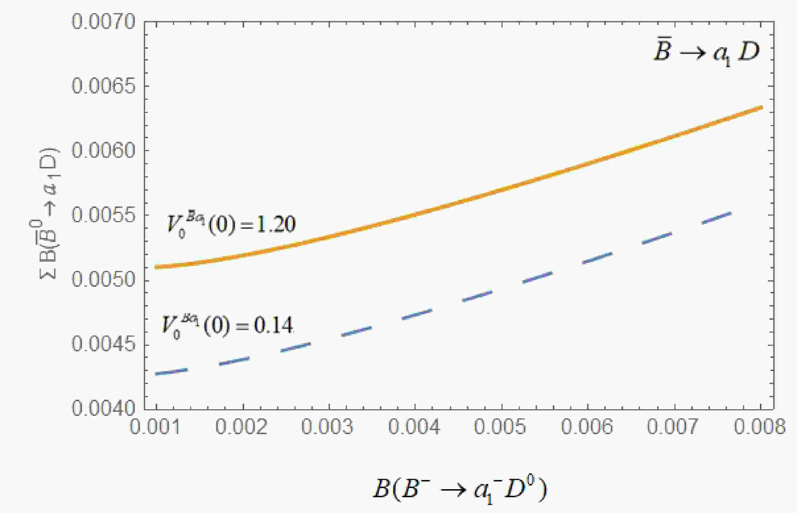
Table 2.  Form-factor of the $ \bar{B} \rightarrow a_{1} $transitions at maximum recoil (q² =0). The results of CQM and QSR have been rescaled according to the form-factor definition.

Considering these uncertainties, in Fig. 1, we present variation of the sum of

Figure 1.  (color online) Variation of $ \sum B\left(\bar{B}^{0} \rightarrow a_{1} D\right) $ with $ B({B^ - } \to {a_1}^ - {D^0}) $ for different values of form-factor.

with respect to $ B({B^ - } \to {a_1}^ - {D^0}) $for different values of form factor, $ {V_0}^{\bar B{a_1}}(0) = 0.14 $ and $ 1.20 $ (the dashed line corresponds to $ {V_0}^{\bar B{a_1}}(0) = 0.14, $ and the solid line corresponds to $ {V_0}^{\bar B{a_1}}(0) = 1.20 $), which enhances our prediction by a factor of $ 1.19, $ i.e.,

We also notice that the present data favour $ B(B^{-} \rightarrow a_{1}^{-} D^{0}) $ being on the higher side. A new measurement of branching fractions of these decays would clarify the situation.

3. $ \bar{B} \rightarrow \pi D_{1}(2.420) $ decay mode

We start by writing the generic formula explicitly for $ {B^ - } \to {\pi ^ - }{D_1}(2.420)_{}^0 $

We take $ \alpha \equiv \dfrac{{A_{1/2}^{nf}}}{{A_{3/2}^{nf}}} = 0.22 $ from the analysis of s-wave meson emitting decays of $ B $-mesons (23).

From the experimental branching $ B\left(B^{-} \rightarrow \pi^{-} D_{1}^{0}\right)= (1.5 \pm 0.6) \times 10^{-3} $ , we get

Now, we obtain factorizable amplitudes for $ {\bar B^0} - $ decays as follows:

where the decay constants are given by

and

are taken from [42]. Required $\bar B \to D_1 $ form factor is given by

The form-factors $ V_{0}^{\bar B D_{1}^{1 / 2}}\left(m_{\pi}^{2}\right) $ and $ V_{0}^{\bar B D^{3/ 2}_1}\left(m_{\pi}^{2}\right) $ are taken from CLFQM [40] results with the following $ q^{2} $ dependence:

where

The $ \bar{B} \rightarrow \pi $form factor,

has already been used in (18). For the charm meson mixing angle $ {\theta _1} = - {(5.7 \pm 2.4)^ \circ } $, we predict,

Here, we also plot variation of the sum of $ B({\bar B^0} \to {\pi ^ - }D_1^{\; + }) $ and $ B({\bar B^0} \to {\pi ^0}D_1^{\;0}) $ with respect to $ B\left(B^{-} \rightarrow \pi^{-} D_{1}{ }^{0}\right) $ in Fig. 2, in the light of experimental error in $ B\left(B^{-} \rightarrow \pi^{-} D_{1}{ }^{0}\right) . $

Figure 2.  (color online) Variation of $ \sum B\left(\bar{B}^{0} \rightarrow \pi D_{1}\right) $ with $ B\left(B^{-} \rightarrow \pi^{-} D_{1}^{0}\right) $.

4. $ \bar{B} \rightarrow \pi D_{1}^{\prime}(2.427) $ decay mode

The generic formula for $ {B^ - } \to {\pi ^ - }{D^{'}}_1(2.427)_{}^0 $ takes the following form:

Here, we also take $ \alpha \equiv \dfrac{{A_{1/2}^{nf}}}{{A_{3/2}^{nf}}} = 0.22 $.

Using experimental branching $B\left(B^{-} \rightarrow \pi^{-} D_{1}^{\prime} (2.427)^{0}\right) \times B\left(D_{1}^{\prime}(2.427)^{0} \rightarrow \pi^{-} D^{*-}\right)$ given in Table 1, assuming that the $ D'^0_{1} $ width is saturated by $ \pi D^{*} $ [50] and then using isospin sum rule,

we obtain $ B\left(B^{-} \rightarrow \pi^{-} D_{1}^{\prime 0}\right)=(7.5 \pm 1.7) \times 10^{-4} $, which yields

Now, we obtain factorizable amplitudes for $ {\bar B^0} - $decays, given by

Here,

We use numerical values for the decay constants and form-factors, as presented in the previous case. Finally, we predict

Considering the uncertainty of the experimental branching $ B\left(B^{-} \rightarrow \pi^{-} D_{1}^{\prime}(2.427)^{0}\right) $, here, we also plot the variation of $ \sum {B\left( {{{\bar B}^0} \to \pi D_1^{'\;}} \right)} $ with respect to $B\left(B^{-} \rightarrow \pi^{-} D_{1}^{' 0}\right)$ in Fig. 3.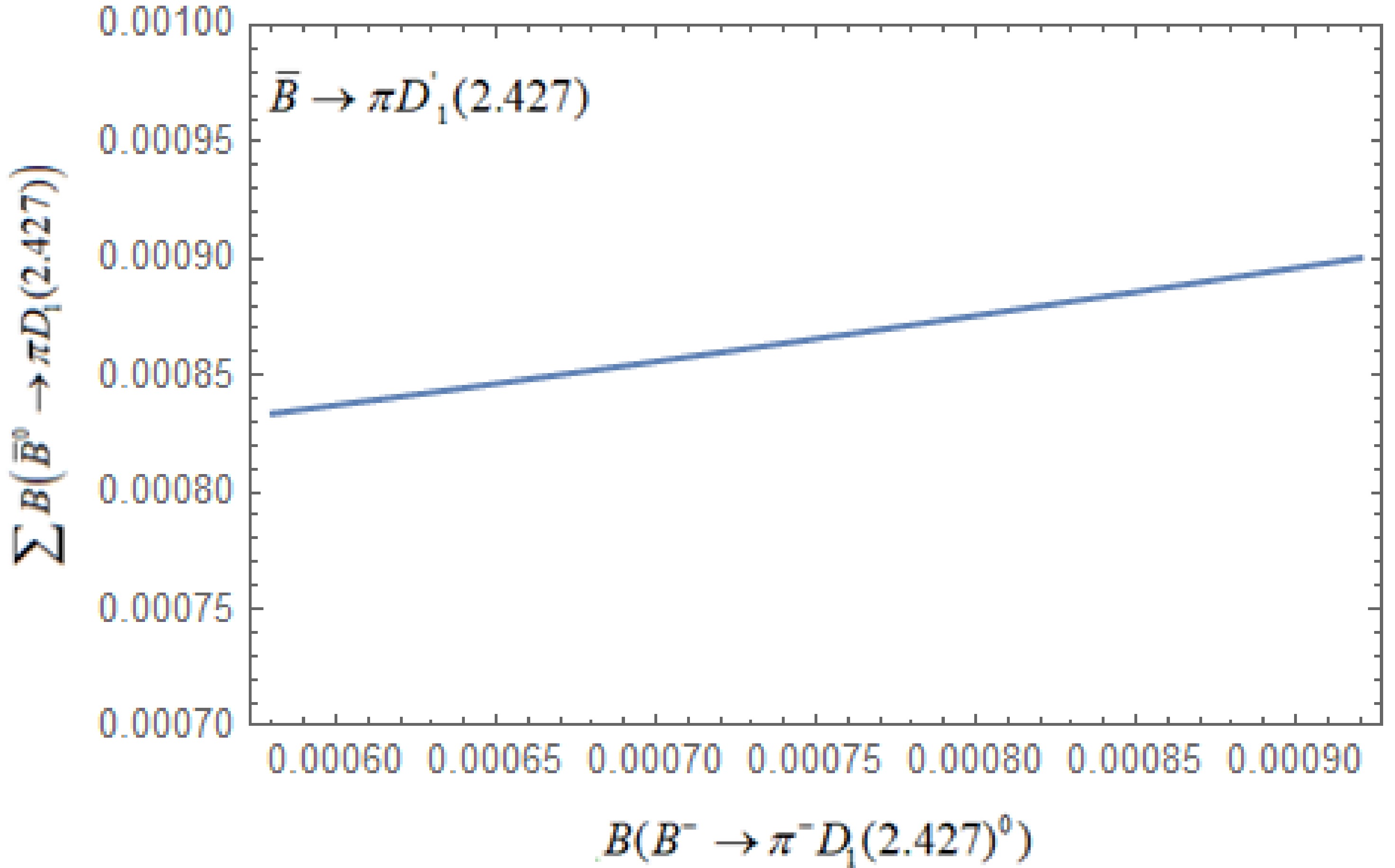

Figure 3.  Variation of $ \sum B\left(\bar{B}^{0} \rightarrow \pi D_{1}^{\prime}\right) $ with $ B\left(B^{-} \rightarrow \pi^{-} D_{1}^{\prime}{ }^{0}\right) $.

Experimentally [1], the tensor meson sixteen-plet comprises of isovector $ {a_2}(1.320), $ strange iso-spinor $ K_2^*(1.430), $ charm triplet $ D_2^*(2.460),\,\;D_{s2}^*(2.573), $ and three isoscalars $ {f_2}(1.270),\,\;f_2^{'}(1.525),\,\; $ and $ {\chi _{c2}}(1P). $ These states behave well with respect to quark model assignments. For $ \bar B \to PT $ decays, only one mode has been observed [1], $ B({B^ - } \to {\pi ^ - }D_2^{*0}(2.460)), $ and more data are expected to come in near future.

The generic formula for $ \bar B \to \pi {D^*}_2 $ decays is given by

We proceed to calculate various quantities on the right-hand side. We combine both the results given in Table 1, i.e.,

to arrive at

Using $ B\left(D_{2}^{*}(2.462)^{0} \rightarrow \pi^{-} D^{+}, \pi^{-} D^{*+}\right) $ = 2/3 following from the isospin symmetry and assuming that the $ D_{2}^{* 0} $ width is saturated by $ \pi D $ and $ \pi D^{*} $ [50−59], we get

We use the branching fraction formula

where p is the magnitude of the three-momentum of the final-state particle in the rest frame of B-meson and m_B and m_T denote masses of the B-meson and tensor meson, respectively.

By using the experimental value (72), we get

The factorization parts of the weak decay amplitudes for $ \bar{B} \rightarrow P T $decays are expressed as the product of matrix elements of weak currents (up to the weak scale factor of $ \frac{G_{F}}{\sqrt{2}} \times\rm C K M \text { elements } \times Q C D \text { factors } $):

The matrix elements $ \left\langle {P} \mathrel{\left | {\vphantom {P {\left. {{J^\mu }} \right|0}}} \right. } {{\left. {{J^\mu }} \right|0}} \right\rangle $ and $ \left\langle {P} \mathrel{\left | {\vphantom {P {\left. {{J_\mu }} \right|B}}} \right. } {{\left. {{J_\mu }} \right|B}} \right\rangle $ are given below. The hadronic current creating meson from the vacuum is given by

where $ {P_B} $ is the four-momentum of the pseudoscalar meson. However, the matrix elements $ \langle T| J^{\mu}|0\rangle $ vanish due to the tracelessness of the polarization tensor $ \varepsilon_{\mu \nu} $ of spin 2 meson and the auxiliary condition $ q^{\mu} \varepsilon_{\mu \nu}=0 $ [60]. Thus, the tensor meson cannot be produced from the V-A current. Relevant B → T matrix elements are expressed as follow:

in the ISGW2 model [5]. The matrix elements simplify to

where

Now, we obtain factorizable amplitude values for $ {\bar B^0} - $decays,

using the decay constant values $ {f_\pi } = - ( 0.131 \pm 0.002 )\;{\text{GeV}} $, as already used in the previous sections [40], and the form factor $ F^{\bar B D_{2}}\left(m_{n}^{2}\right)=0.52,0.38, $ taken from the CLFQM [40] and ISGW models [3]:

$ A^{f}\left(\bar{B}^{0} \rightarrow \pi^{0} D_{2}^{* 0}\right) $becomes zero due to vanishing of the decay constant of the $ D_{2}^{*} $ meson. Finally, using (69) for $ \alpha = 0.22 $, we predict

for the two choices of $ F^{\bar B D_{2}}\left(m_{n}^{2}\right)=0.52,\,0.38, $ respectively, which may be tested in future experiments. Considering the ambiguity of the experimental $ B(B^{-} \rightarrow \pi^{-} D_{2}^{*}(2.460)^{0}), $ we show the increasing behavior of $ \sum B\left(\bar{B}^{0} \rightarrow \pi D_{2}\right) $ with respect to$ B\left(B^{-} \rightarrow \pi^{-} D_{2}^{* 0}\right) $ in Fig. 4 for both choices, shown as dashed and thick lines, respectively.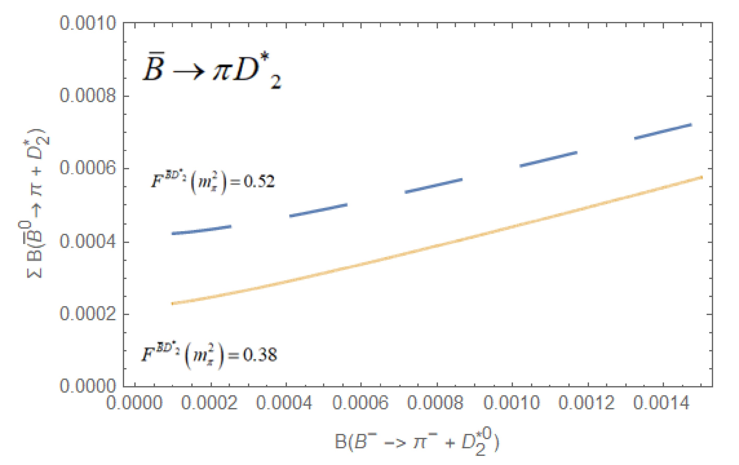

Figure 4.  (color online) Variation of $ \sum {B\left( {{{\bar B}^0} \to \pi \;D_2^*} \right)} $ with $ B({B^ - } \to {\pi ^ - }\;D_2^{*\;0}) $ for different values of form-factor.

The scalar mesons mostly appear as the hadronic resonances and have large decay widths. There will exist several resonances and decay channels within a short mass interval. The overlaps between resonances and background make it considerably difficult to resolve the scalar mesons. The scalar-meson family has been the most difficult one to identify as a standard sixteen-plet. Experimentally [1], the following states of scalar meson sixteen-plet, isovector $ {a_0}(0.980), $ strange spinor $ K_0^*(1.429), $ one isoscalar $ {\chi _{c0}}(1P)(3.145), $and charm triplet $ D_0^*(2.400),\; D_{s0}^*(2.480), $ behave well with respect to quark model assignments. For $ \bar B \to PS $ decays, only one mode has been observed [1], $ B({B^ - } \to {\pi ^ - }D_0^{*0}(2.400)), $ and more data are expected to come in the near future.

Writing the generic formula explicitly for $ \bar B \to \pi D_0^* $ decays,

To obtain the branching fraction $ B\left(B^{-} \rightarrow \pi^{-} D_{0}^{* 0}\right) $ from the experimental value

given in Table 1, we employ isospin symmetry, which gives

and realizing the saturation of strong $ D_{0}^{* 0} $ decays with $ D_{0}^{* 0} \rightarrow \pi D $ modes [52], we estimate

for our analysis. Using this estimate and decay rate formula, similar to that of $ \bar{B} \rightarrow P P, $

and we get

We then obtain factorizable amplitudes for $ {\bar B^0} - $decays, which are given as

Numerical values are calculated using the decay constants [42],

and $ F^{\bar B D_{0}^{*}}\left(m_{\pi}^{2}\right) $from the CLFQM [40] results, i.e.,

where

and the form-factor $ F^{\bar B \pi}(0)=0.27 \pm 0.05 $ was already given in previous sections.

Finally, we predict

for $ \alpha = 0.22\;. $ Here, we also plot the variation of $ \sum {B\left( {{{\bar B}^0} \to \pi {D_0}^*} \right)} $ with respect to $ B\left(B^{-} \rightarrow \pi^{-} D_{0}^{* 0}\right) $ in Fig. 5, which also shows increasing behaviour.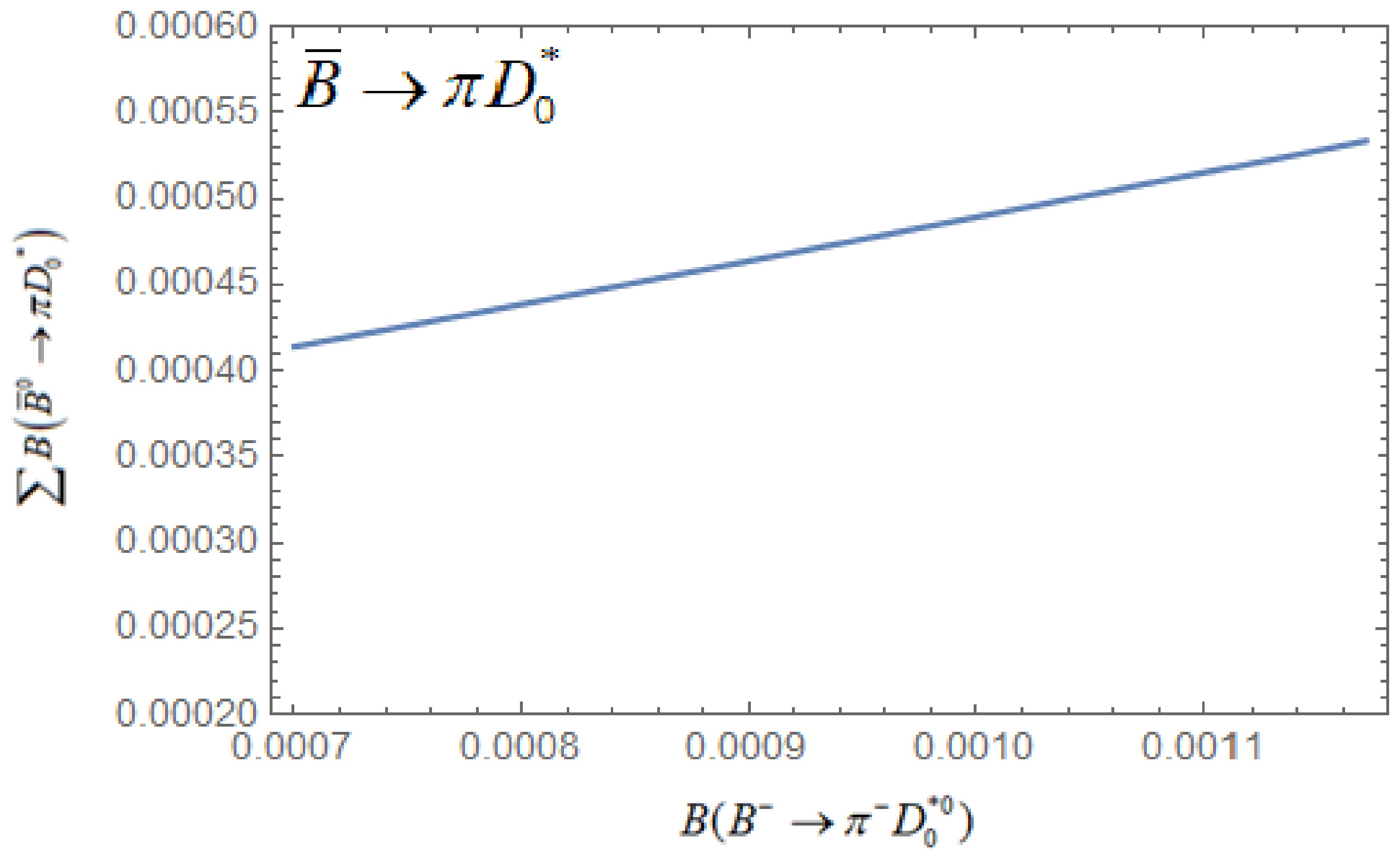

Figure 5.  (color online) Variation of $ \sum B\left(\bar{B}^{0} \rightarrow \pi D_{0}^{*}\right) $ with $ B\left(B^{-} \rightarrow \pi^{-} D_{0}^{* 0}\right) $.

In our previous work, we conducted isospin analysis of CKM-favored two-body weak decays of bottom mesons $ \bar B \to PP/PV, $occurring through W-emission quark diagrams. Obtaining the factorizable contributions from the spectator-quark model for N_c = 3 (real value), we have determined nonfactorizable reduced isospin amplitudes from the experimental data for these modes. We have observed that in all the decay modes, the nonfactorizable isospin reduced amplitude $ A_{1/2}^{nf} $ bears the same ratio as$ A_{3/2}^{nf} $ within the experimental errors. In the charm sector, a systematics observed for the charm mesons decaying to s-wave mesons has been found to be consistent with their p-wave meson emitting decays [22]. Encouraged by the success for the s-wave emitting decays in the bottom meson sector [36], we have extended isospin analysis to the p-wave meson emitting decays in $ \bar B \to PA/ PT/PS $ channels, particularly for the $ \bar B \to {a_1}D/\pi {D_1}/\pi {D'_1}/ \pi {D_2}/\pi {D_0} $ decays, which have the same isospin structure as that of $ \bar B \to \pi D/\rho D/\pi {D^*} $ cases.

To include the effects of nonfactorizable contributions, for these cases, we exploit the generic formula to predict the sum of the branching fractions of $ {\bar B^0} - $ decays in these channels. As there are large errors involved in $ B(\bar B \to {a_1}D) = (4 \pm 4) \times {10^{ - 3}} $ and the form-factor $ F^{\bar B a_1}(0) $ is not uniquely known, looking at these uncertainties, we plot the variation of $ \sum B\left(\bar{B}^{0} \rightarrow { deccys }\right) $ with respect to $ B({B^ - } \to {a_1}^ - {D^0}) $ for extreme values of $ {V_0}^{\bar B{a_1}}(0) = 0.14 $ and 1.20, which enhances our prediction by a factor of 1.19. Our predictions will be tested in future experiments.

We extend our analysis to $ \bar B \to \pi {D_1}/\pi {D^{'}}_1/\pi {D_2}/\pi {D_0} $ decay modes, which have a similar isospin structure, and make predictions for $ {\bar B^0} - $decays. It is hoped that the predictions made in this paper will help experimentalists to identify the p-wave meson emitting decays of the heaviest bottom mesons.