Primordial black holes and scalar induced density perturbations: the effects of probability density functions

In inflation theory, valuable information about the early Universe is encoded in the cosmological perturbations that originated from the quantum fluctuations during inflation. The power spectrum of primordial curvature perturbations $ \mathcal{P}_{\zeta}\left(k \right) $ is one of the most important predictions in inflation theory. The amplitude of the primordial power spectrum at different scales can be constrained by current cosmological observations. On large scales ($ \gtrsim $1 Mpc), according to the current observations of the CMB and LSS [1, 2], the amplitude of the power spectrum of primordial curvature perturbations is constrained to be approximately $ 2\times 10^{-9} $. However, on small scales ($ \lesssim $1 Mpc), the constraints of primordial curvature perturbations are significantly weaker than those on large scales [3]. Constraining the primordial power spectrum on small scales is an important issue in the study of the early Universe.

Two approaches are adopted to constrain or probe the primordial power spectrum on small scales: primordial black hole (PBH) abundance and scalar induced gravitational waves (SIGWs). More precisely, the large amplitudes of the small-scale primordial spectrum have attracted significant attention in the past few years on account of their rich and profound phenomenology, such as the PBH [4−28], which is a candidate of DM. The abundance of PBHs, $ f_{\mathrm{pbh}} $, can be calculated in terms of a given primordial power spectrum of curvature perturbation, $ \mathcal{P}_{\zeta}(k) $. The abundance of PBHs, $ f_{\mathrm{pbh}}(m_{\mathrm{pbh}}) $, has been constrained on different masses of PBHs, $ m_{\mathrm{pbh}} $ [8, 29]; then, the corresponding small-scale primordial power spectrum can also be constrained by various observations of PBHs. Furthermore, the primordial perturbations will inevitably generate higher order perturbations, such as SIGWs [28, 30−60]. This strong correlation between primordial curvature perturbation and SIGW signals might be a promising approach to detecting a small-scale primordial power spectrum in the GW experiments, such as LISA and PTA [60−74].

In this study, we investigate the contributions of second order induced energy density perturbations, $ \delta^{(2)}= \rho^{(2)}/\rho^{(0)} $, to the PBH formation. More precisely, the primordial curvature perturbation that enters the Hubble radius during the radiation-dominated (RD) era will lead to the generation of higher order scalar and energy density perturbations. Then, the relative abundance of PBHs can be studied in terms of the probability density functions (PDFs) of the total energy density perturbations: $P\left(\delta^{(1)}+\delta^{(2)}/{2}\right)$, where $ \delta^{(1)} $ denotes the contributions of the primordial curvature perturbation which have been studied for many years [9, 75]. Here, $ \delta^{(2)} $ is the new contribution of the second order scalar induced energy density perturbation $ \delta^{(2)} $, which was neglected in previous studies of PBHs ¹. Because the abundance of PBHs, $ f_{\mathrm{pbh}}(m_{\mathrm{pbh}}) $, has been constrained on different $ m_{\mathrm{pbh}} $, the amplitude of small-scale primordial power spectra can be constrained by the abundance of PBHs.

This paper is organized as follows. In Sec. II, we calculate the second order scalar induced density perturbation in the comoving gauge. In Sec. III, we study the impact of second-order scalar-induced density perturbations on the PDF and discuss the constraints on the PBH abundance imposed by the small-scale primordial power spectrum. Finally, we summarize our results and present some discussions in Sec. IV.

The perturbed metric in the FLRW spacetime with the comoving gauge takes the form

where $ \phi^{(n)} $, $ \psi^{(n)} $, and $ B^{(n)} $$ (n=1,2) $ are the nth-order scalar perturbations. We set the n-th order perturbation of the scalar part of the velocity, $ \delta u^{(n)}=0 $, and the scalar metric perturbation, $ E^{(n)}=0 $, in the comoving gauge. In the radiation dominated (RD) era, the first order scalar perturbation is given by

where $ \zeta_{\mathbf{k}} $ denotes the primordial curvature perturbations. The transfer functions $ T_\phi(k \eta), T_\psi(k \eta) $, and $ T_B(k \eta) $ in the RD era are [76]

where we define $ x \equiv k \eta $. The higher order cosmological perturbations can be studied in terms of the $\mathrm{xPand}$ package [77, 78]. The equations of motion of second order scalar perturbations are

where $ S^{(2)}_{ij} $ and $ S^{(2)}_{i} $are second order source terms

$ \mathcal{T}^{ij} $ is defined as $ \mathcal{T}^{ij}=\delta^{ij}-\partial^{i} \Delta^{-1} \partial^{j} $. The second order energy density perturbations $ \delta^{(2)}=\rho^{(2)}/\rho^{(0)} $ can be calculated in terms of second order induced scalar perturbations and first order scalar perturbations,

where $ S^{(2)}_{\rho} $ are given by

As the large-amplitude primordial curvature perturbations $ \zeta_{\mathbf{k}} $ on small scales are necessary for the formation of PBHs, we consider the log-normal primordial power spectrum

In the limit of $ \sigma_* \rightarrow 0 $, $ \mathcal{P}_{\zeta}(k) $ approaches to a monochromatic power spectrum, namely, $ \mathcal{P}_{\zeta}(k)=A_\zeta k_* \delta\left(k-k_*\right) $.

In previous studies on PBHs, the PDF of the primordial curvature perturbation $ \zeta_{\mathbf{k}} $ was often assumed to be Gaussian, resulting in a Gaussian PDF for the first order energy density perturbation $ \delta^{(1)} $ [75]. In this study, we consider the contribution of second order scalar induced energy density perturbations $ \delta^{(2)} $to the formation of PBHs. As we mentioned, the statistics of second order scalar induced energy density perturbations are highly non-Gaussian. Therefore, the PDFs of the total energy density perturbation $\delta_r=\delta^{(1)}+\dfrac{1}{2}\delta^{(2)}$ cannot be directly and simply obtained. We follow the method described in Ref. [58] to calculate the highly non-Gaussian PDFs of $ \delta_r $. In Ref. [58], the PDFs of the second order energy density perturbation induced by primordial gravitational waves were studied. Here, we calculate the PDFs of the total energy density perturbation $\delta_r=\delta^{(1)}+\dfrac{1}{2}\delta^{(2)}$ induced by primordial curvature perturbations $ \zeta_{\mathbf{k}} $. The relation between $ \delta_r $ and $ \zeta_{\mathbf{k}} $ can be rewritten as

where $ W(x)=3\left(\sin x-x\cos x \right)/x^3 $ is the window function [58]. $ I_{\delta^{(2)}} $ is the kernel function of $ \delta^{(2)} $ ², and $ \mathcal{P}_{\zeta} $ is the log-normal primordial power spectrum. Eq. (10) describes the relationship between the random variables $ \delta_r $ and ζ. The PDF of $ \delta_r $ (non-Gaussian distribution) can be simulated in terms of the PDF of ζ. The mass-scale relation of PBHs can be expressed as follows [58]:

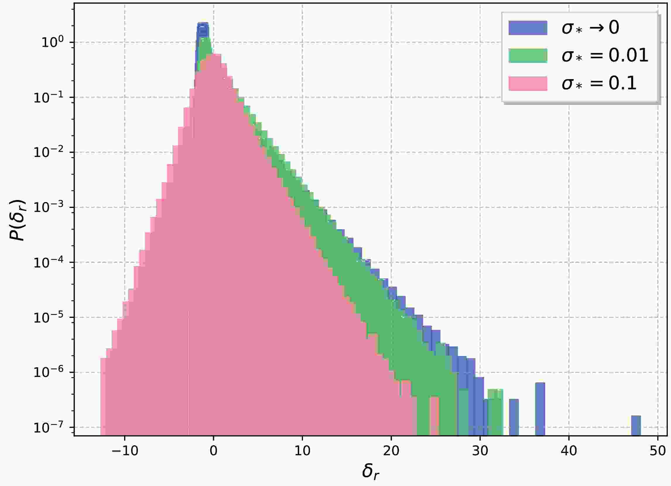
To intuitively show the trend of the PDFs with respect to $ \sigma_* $, we calculate the PDFs corresponding to different $ \sigma_* $ values near $ \sigma_*=0 $. As shown in Fig. 1, the PDFs of $ \delta_r $ are highly non-Gaussian and contract gradually as $ \sigma_* $ increases. Therefore, relying solely on the variance, $ \sigma^2 $, is insufficient to evaluate the probability of PBH formation. In this study, we calculate the PDF function corresponding to different values of η within the range $ [0.2, 10] $. As in Ref. [58], we select the moment that yields the maximum number of PBHs, resulting in a final η of approximately 0.4. The relative abundance of PBHs $ f_{\mathrm{pbh}}(m_{\mathrm{pbh}}) $ is equivalent to the probability that the smoothed density field exceeds the threshold $ \delta_c $ [75, 79],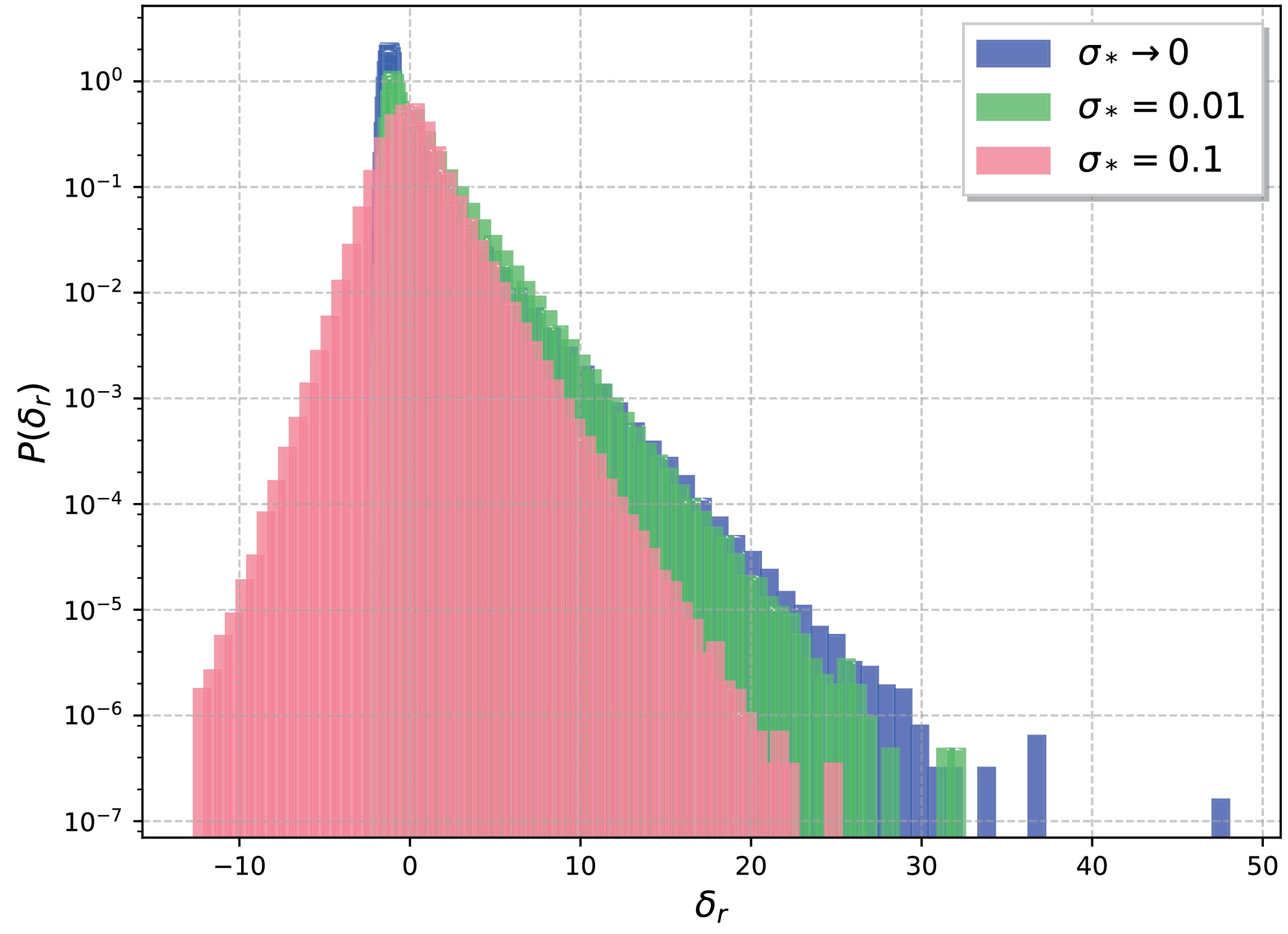

Figure 1.  (color online) PDFs of the total energy density perturbation $ \delta_r=\delta^{(1)}+\frac{1}{2}\delta^{(2)} $ for a log-normal primordial power spectrum with different $ \sigma_* $, where we set $ A_\zeta = 1 $ and $ \eta\approx0.4 $.

where the value of the threshold $ \delta_c $ is, in fact, influenced by the characteristics of the primordial perturbation (its shape and the degree of non-Gaussianity). In reality, this value may vary significantly depending on these properties [80−84]. Here, we are primarily concerned with the impact of introducing second-order density perturbations on the PDF of the final density perturbation. It is important to emphasize that our calculation of the PDF here does not depend on the choice of the threshold $ \delta_c $. For simplicity, we have set $ \delta_c = 0.4 $.

By substituting the PDF $ P\left(\delta^{(1)}+\frac{1}{2}\delta^{(2)}\right) $ of the total energy density perturbations into Eq. (12), we obtain $ \beta(A_{\zeta}) $ as a function of $ A_{\zeta} $ (Fig. 2). As β has been constrained at different masses of PBHs, we use Fig. 18 in Ref. [8] to determine the upper bounds of $ A_{\zeta} $. As shown in Fig. 3, for a log-normal primordial power spectrum, its amplitude $ A_{\zeta} $ is constrained to be approximately $ A_{\zeta}\sim 3\times10^{-3} $. The local-type non-Gaussian primordial curvature perturbation is given by [85, 86]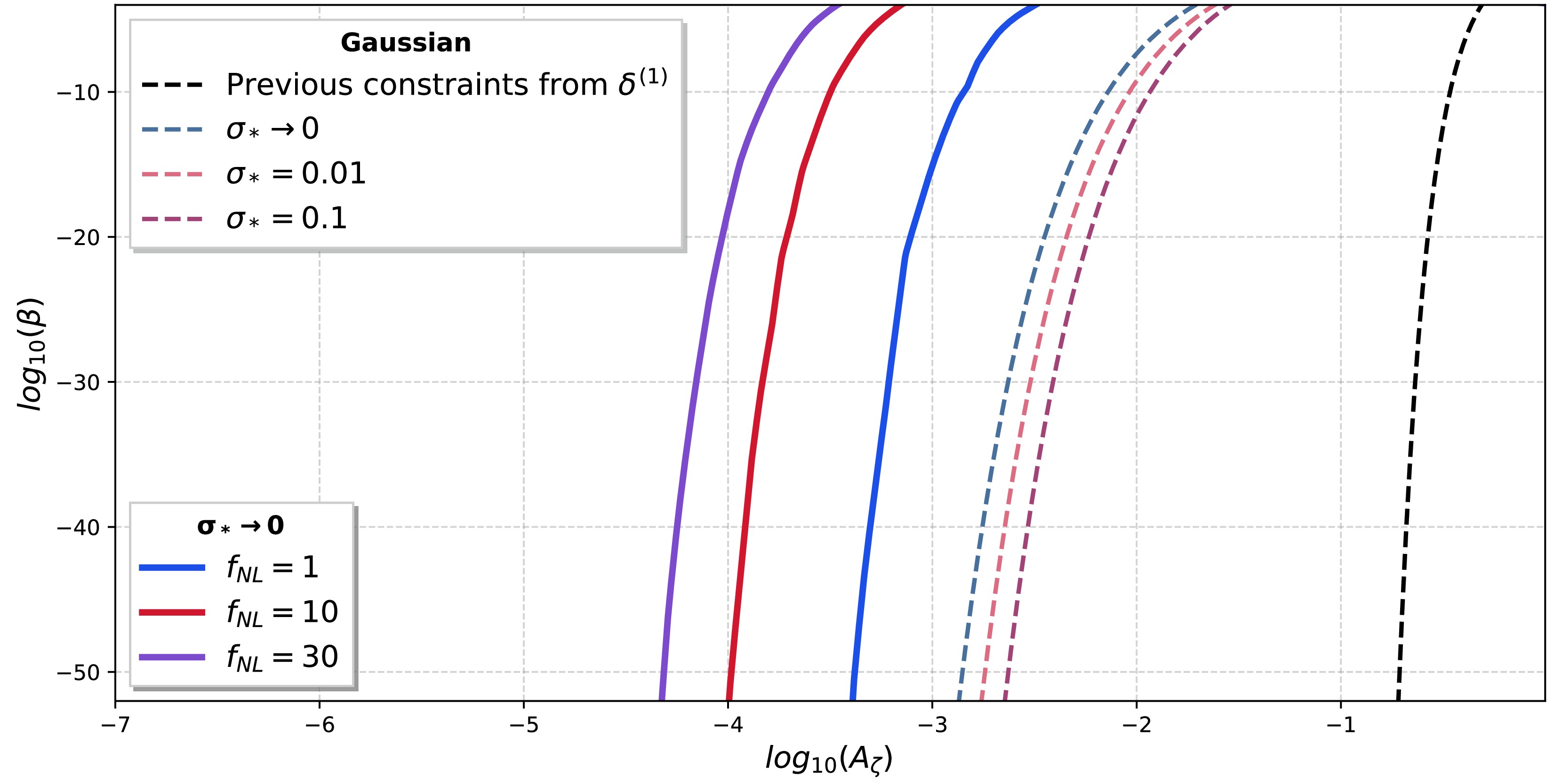

Figure 2.  (color online) Primordial black hole abundance β as a function of the amplitude of the primordial power spectrum $ A_\zeta $. The three colored dashed lines represent the relations between β and $ A_{\zeta} $ for different $ \sigma_* $values. The three solid lines represent $ \beta(A_{\zeta}) $ for the local-type non-Gaussian primordial curvature perturbations $\zeta^{\rm NG}_{\mathbf{k}}$ with different $ f_{\mathrm{NL}} $values. The black dashed line represents the previous results from $ \delta^{(1)} $ in Ref. [75].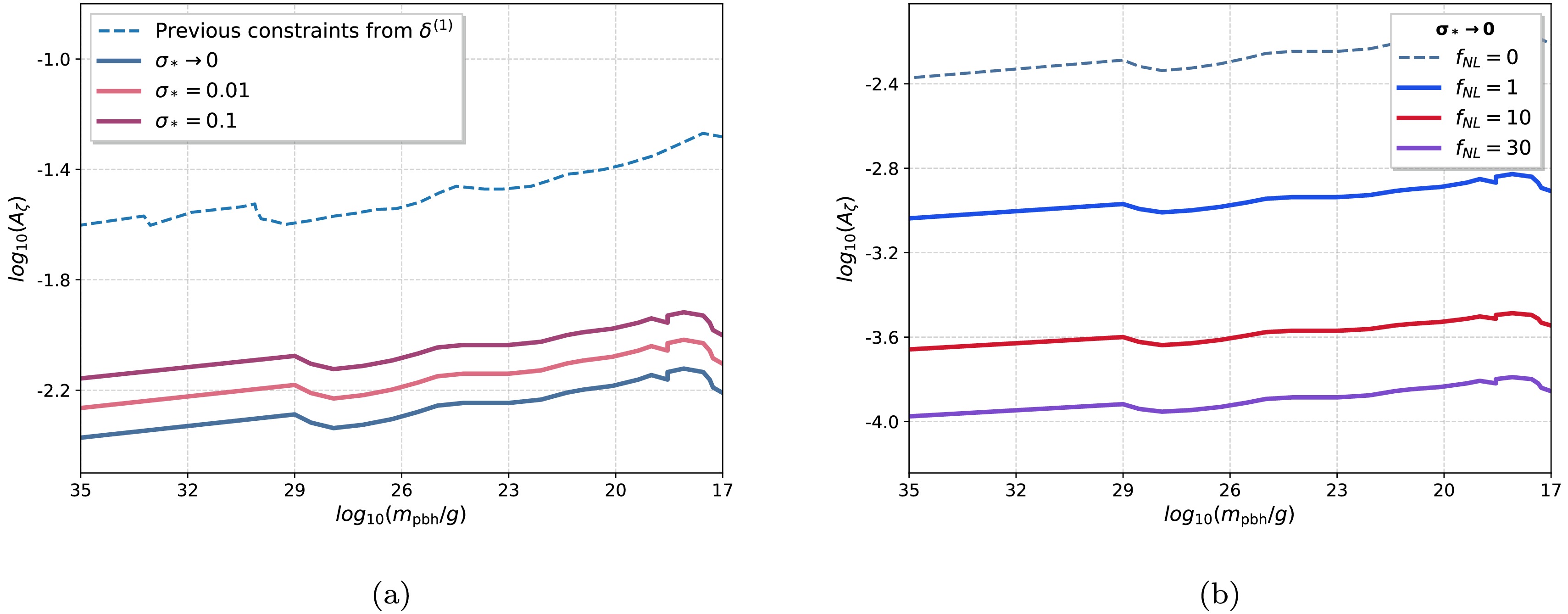

Figure 3.  (color online) Left panel: Upper bounds of $ A_{\zeta} $ from the total energy density perturbation $ \delta_r $ with different $ \sigma_* $ values. The blue dashed line represents the previous results from $ \delta^{(1)} $ in Ref. [75]. Right panel: Upper bounds of $ A_{\zeta} $ for different $ f_{\mathrm{NL}} $ values. The dashed line represents the case of a Gaussian primordial curvature perturbation.

where $ \zeta^G $ is the Gaussian primordial curvature perturbation. Here, we consider the lowest order contributions of local-type non-Gaussianity, namely, $ \delta^{(1)}_{NG}\sim A_{\zeta}f_{\mathrm{NL}} $ and $ \delta^{(2)}_{NG}\sim A^{3/2}_{\zeta}f_{\mathrm{NL}} $. As shown in Fig. 2, in this case, $ \beta\left(A_{\zeta},f_{\mathrm{NL}} \right) $ is a function of $ A_{\zeta} $ and $ f_{\mathrm{NL}} $. The upper bounds of $ A_{\zeta} $ with different $ f_{\mathrm{NL}} $ values are given in Fig. 3(b). For $ f_{\mathrm{NL}}=10 $, the upper bound of $ A_{\zeta} $ is approximately $ 2.5\times10^{-4} $. When we consider the second order induced energy density perturbation, the effects of primordial non-Gaussianity will greatly reduce the upper bounds of $ A_{\zeta} $, even for a relatively small $ f_{\mathrm{NL}} $.

In this study, we analyzed the new effects of second order scalar induced energy density perturbation $ \delta^{(2)} $ on PBH formation. We calculated PDFs and β as a function of $ A_{\zeta} $ and $ \sigma_* $ in terms of the log-normal primordial power spectra, where we selected the threshold $ \delta_c=0.4 $ for convenience. In order to not overproduce PBHs, the parameters of primordial power spectra were constrained. For $ \sigma_* \to 0 $, the amplitude of primordial power spectra was constrained to be approximately$ A_{\zeta}\sim 3\times10^{-3} $. With the increase in $ \sigma_* $, the upper bounds of $ A_{\zeta} $ gradually increased. The local-type non-Gaussianity was also considered in this study. For $ f_{\mathrm{NL}}=10 $, the upper bound of $ A_{\zeta} $ was approximately $ 2.5\times10^{-4} $. The effects of primordial non-Gaussianity greatly reduced the upper bounds of $ A_{\zeta} $, even for a relatively small $ f_{\mathrm{NL}} $. In addition, as the upper bound of $ A_{\zeta} $ was constrained to be approximately $ A_{\zeta}\sim 3\times 10^{-3} $ for a Gaussian primordial curvature perturbation, the energy density of third order SIGWs was always less than that of second order SIGWs.

The relative abundance of PBHs $ f_{\mathrm{pbh}}(m_{\mathrm{pbh}}) $ depends on the probability that the smoothed density field exceeds the threshold $ \delta_c $ [79], namely, $\beta\left(M_{\mathrm{PBH}}\right)= \int_{\delta_c} {\rm d} \delta_r P(\delta_r)$.To investigate the impact of second order induced density perturbation $ \delta^{(2)} $ on β, we first need to calculate the corresponding PDFs and the threshold $ \delta_c $. The calculation of the threshold $ \delta_c $ is quite complex, as it depends on the shape of the primordial power spectrum and the specific PBH model under consideration. In this study, we treated the threshold $ \delta_c $ as a fixed parameter, focusing on the impact of second-order scalar-induced density perturbations on the PDFs. The effects of higher-order density perturbations on the threshold $ \delta_c $ may be studied in future work.

We acknowledge the $\mathrm{xPand}$ package [77].