Quasinormal modes of a black hole surrounded by a fluid of strings in Rastall gravity

General relativity has withstood extensive scrutiny since its predictions were first confirmed in 1919, particularly through phenomena like the deflection of light by the Sun. Recent evidence from gravitational wave observations by LIGO and Virgo further supports its robustness [1−3]. However, general relativity does not account for dark matter and energy or the cosmic acceleration [4, 5], and it is not renormalizable [6]. These limitations motivate the exploration of modified theories, of which Rastall gravity is one [7]. Rastall proposed a modification to the energy-momentum conservation law, suggesting that its divergence could be proportional to the gradient of the Ricci scalar [7]. This leads to a non-minimal coupling of matter with spacetime geometry, recovering standard conservation in flat spacetime. Numerous studies have suggested that Rastall gravity is a viable alternative, with applications in astrophysics and cosmology [8−15]. Notably, solutions involving black holes surrounded by a cloud of strings have been explored, revealing interesting properties, such as critical rotation parameters for extremal black holes [16] and the stability of certain gravastar models [17]. The concept of a string cloud as a source of gravitational fields dates back to Letelier, who developed solutions to the Einstein equations for various symmetries [18, 19]. This laid the groundwork for later studies that incorporated pressure effects [20] and anisotropic fluids [21−23]. The potential of Rastall gravity to modify spacetime properties makes it a compelling area for further investigation, especially in conjunction with models involving strings.

Recent interest in Rastall gravity has surged, driven by its ability to reconcile certain astrophysical observations, such as the dynamics of dark energy and cosmic acceleration, without invoking dark matter [24]. Its field equations can describe a variety of interesting solutions, including those of black holes surrounded by fluids or exotic matter, thus broadening our understanding of gravitational interactions. Notably, Rastall gravity can yield unique behaviors not present in general relativity, such as alterations in the quasinormal modes (QNMs) of black holes and novel stability conditions. The theory also exhibits compatibility with certain cosmological models, presenting potential explanations for observed cosmic phenomena [24, 25]. Given these compelling features, Rastall gravity stands as a fruitful area of research, especially regarding its implications for black hole physics and the nature of gravitational interactions in the universe.

QNMs are essential characteristics of dissipative systems, particularly in black holes, where anything that crosses the event horizon cannot escape. QNMs dominate the ringdown phase of gravitational waves from binary black hole mergers [26]. Unlike those of normal modes, the eigenfunctions of QNMs do not form a complete set and are not normalizable [27]. QNMs exhibit complex frequencies, with real parts representing vibration frequencies and imaginary parts indicating decay time scales. Studying QNMs is crucial for inferring the mass and angular momentum of black holes, as well as testing the no-hair theorem [28−30]. In horizonless compact objects, QNMs may reveal echoes in the ringdown signal, providing evidence for their existence [31−33]. Additionally, QNMs can constrain modified gravity theories [34−42] and have been found to be unstable under small potential perturbations [43, 44]. They also help assess the stability of the background spacetime under perturbations [45, 46]. Researchers have explored the impacts of different parameters on QNM behavior and stability in various black hole spacetimes, including those under the influence of magnetic fields, regular black holes, high-dimensional noncommutative black holes, and noncommutative black holes coupled to Einstein's tensor [47−50].

In this paper, we focus on the black hole surrounded by a fluid of strings in Rastall gravity, as presented in Ref. [51]. We investigate the QNMs of the Rastall black hole under three distinct types of perturbations of scalar, electromagnetic, and gravitational fields. We analyze the effects of the black hole parameters on the quasinormal frequencies, revealing how these parameters influence the stability and decay properties of perturbations. The remainder of this paper is organized as follows. First, we review the solutions of a black hole surrounded by a fluid of strings in Rastall gravity in Section II. Then, Sections III and IV give the pertubation equations of three fields and detail our numerical methods for calculating the QNMs. Section V presents the figures of QNMs and discusses our results. Finally, we provide concluding remarks in Section VI.

Considering the modification to the theory of general relativity made by Peter Rastall [7]

where β is a constant and R is the Ricci scalar, the field equation reads as

In the limit as $ \lambda \to 0 $, $ k = 8 \pi G_N $, where $ G_N $ represents the Newtonian gravitational constant, and the field equations reduce to GR field equations.

In four-dimensional spacetime, the energy-momentum tensor $ T_{\mu\nu} $ of perfect fluid reads as [51]

where parameters q and ρ represent the pressure and density of the fluid of strings, respectively.

Then, the solution of a black hole surrounded by a fluid of strings in four-dimensional Rastall gravity is [51]

where

where λ and L are positive constants, and Q represents the electric charge. $ \varepsilon=\pm 1 $ gives the sign of the energy density of the fluid of strings, and A is defined as

where α is a dimensionless constant.

The horizons give us the relationship between black hole mass M and radius $ r_h $

Black hole temperature T can be obtained by the following relation: $ T=\frac{f'(r)}{4\pi} $, which results in

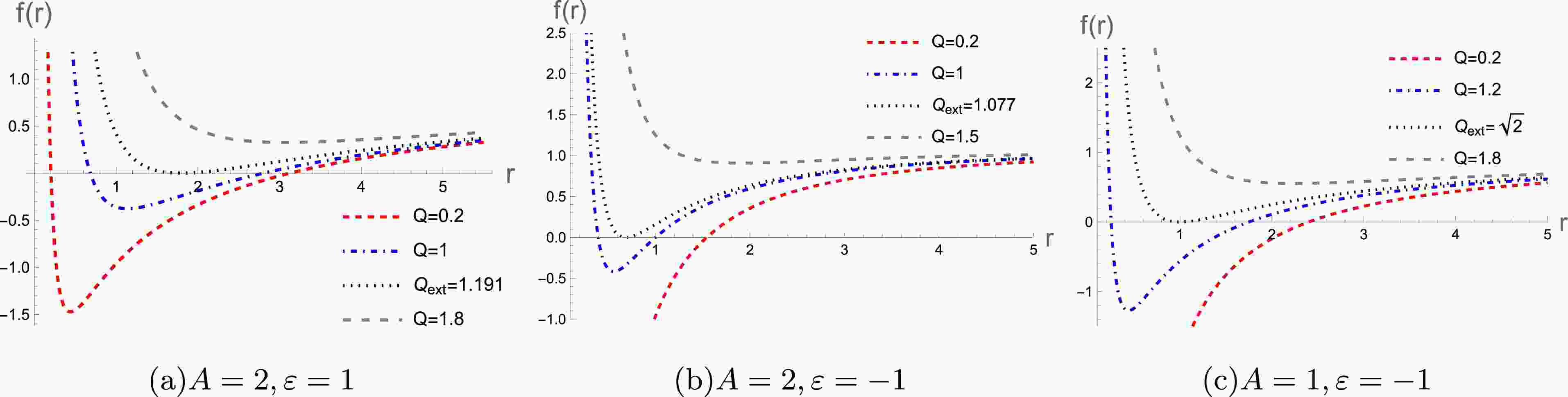
where $ \gamma(r_h)=\varepsilon L/r_h^2 $ for $ A=2 $ and $ \gamma(r_h)=\varepsilon r_h^{-1} (\frac{L}{r_h})^{2/A} $ for $ A \neq 2 $.

Figure 1 shows how varying Q affects the existence of the event horizon, allowing us to give the effective range of Q. For example, the black dotted line marks the extremal value of Q ($Q_{\rm ext}$), where the two horizons of the black hole merge. Figure 2 shows the curves of Hawking temperature as a function of event horizon radius $ r_h $ for different values of A and ε. As the Hawking temperature tends to zero, we can obtain the extreme value of the horizon radius and charge. For example, $A=2,\; \varepsilon=+1$, extreme radius $r_{ h\rm ext}=1.792$, and extreme charge $Q_{\rm ext}= 1.191$ can be calculated by the following equations: $ f(r_h)=0 $ and $ T(r_h)=0 $. Similarly, when $A=2,\; \varepsilon=-1$, we get $r_{h\rm ext}=0.6874$ and $Q_{\rm ext}=1.077$. $A=1,\; \varepsilon=-1$ correspond to $r_{h\rm ext}=1.0$ and $Q_{\rm ext}=\sqrt{2}$.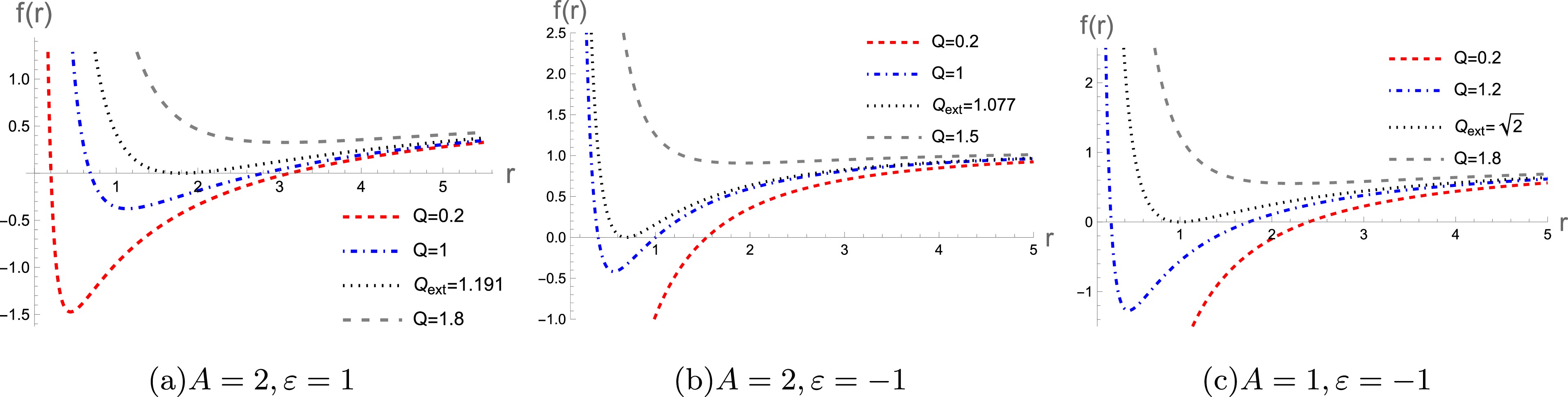

Figure 1.  (color online) Graph of $ f(r) $as a function of r for different values of Q. We chose values $ M=\lambda=L=1 $.

Figure 2.  (color online) Plots of the Hawking temperature as a function of the event horizon radius $ r_h $for different values of A and ε. We chose values $ M=\lambda=L=1 $.

In this section, we examine the linear perturbation equations for the scalar, electromagnetic, and gravitational fields in the background of a black hole surrounded by a fluid of strings in Rastall gravity. For clarity, we consider each type of perturbed field independently, assuming that perturbing one field does not affect the background of the other two fields.

We consider the evolution of a free massless scalar field; the equation for a scalar in the background of this black hole is given by

To perform a separation of variables, we introduce radial function $ \varphi_s(r) $ and spherical harmonics $ Y_{lm}(\theta,\phi) $ as

By substituting Eq. (10) into Eq. (9), the radial perturbed equation can be written in the Schrödinger wavelike form

where "tortoise coordinate" $ r_{*} $ is defined as

The effective potentials of the scalar field are given by

where $l=0,1,2,\cdots$ are the multipole numbers.

The equation for electromagnetic perturbation in the background of this black hole can be written as

where $ F_{\rho\sigma}=\partial_{\rho}A_{\sigma}-\partial_{\sigma}A_{\rho} $, and $ A_{\mu} $ is the field-strength tensor of the perturbed electromagnetic field, which can be decomposed as

Due to the spherical symmetry of the background metric, the perturbation equations separate polar and axial contributions. Furthermore, the axial and polar parts have equal contributions to the final result [52, 53]. Therefore, we only need to focus on the axial part.

By substituting Eq. (15) into Eq. (14), the perturbation equation for the radial function$ \varphi_e(r) $can be written in the Schrödinger wavelike form using tortoise coordinate $ r_* $

where the effective potentials of the electromagnetic field are given by

The EM modes exist for $ l \geq 1 $.

We consider the first-order gravitational perturbed fields around the background quantities

where $ h_{\mu\nu} $ is the perturbation. The separation of perturbations for the gravitational field is more complicated. This decomposition divides the tensor-vector perturbations into "axial (A)" modes, which gain a factor of $ (-1)^{l+1} $ under parity inversion, and "polar (P)" modes, which gain a factor of $ (-1)^{l} $.

Under the Regge–Wheeler gauge [54], we expand the metric perturbations using tensor spherical harmonics. For the axial part (odd parity), which involves two modes $ h_0 $ and $ h_1 $, the perturbed metric is expressed as

For polar perturbations (even parity) with four modes $ (H_0, H_1, H_2, K) $, we have

Note that we can chose $ m=0 $ in the later calculation for simplicity, as the perturbation equations are independent of the value of m [54].

For the Schwarzschild black hole, Ref. [55] showed that the odd and even parities share the same QNM spectrum, though this may not be true for other black holes. In this paper, we simplify our analysis by focusing on the odd parity. By substituting the decomposition into Einstein's equations and performing some algebraic manipulations, the perturbation equations for odd parity can be consolidated into a single equation for variable $ \varphi_{g} $, which can be written as

By substituting Eq. (21) and Eq. (19) into the equations of motion Eq. (2), after some algebraic calculations and simplification, we can obtain the following master perturbation equations in the Schrödinger wavelike form using tortoise coordinate $ r_* $

where the effective potentials of gravitational field are given by

The gravitational modes exist for $ l \geq 2 $.

In recent years, a new method known as the asymptotic iteration method (AIM) [56] has been developed, which demonstrates greater efficiency in certain cases. This method was previously utilized to solve eigenvalue problems as a semi-analytic technique for second-order homogeneous linear differential equations. Some of the current authors have successfully shown that AIM is both efficient and accurate for calculating QNMs.

It is noteworthy that these three types of perturbations—scalar, electromagnetic, and gravitational—exhibit a similar mathematical structure, allowing them to be transformed into a Schrödinger-like form [30]. This inherent similarity in the formulation justifies the use of the same numerical technique, AIM, for their analysis. By employing the AIM across these different perturbations, we can maintain consistency in our calculations while effectively leveraging the advantages of this method in solving the corresponding second-order differential equations.

We are going to employ the improved asymptotic iteration method [56] to solve the perturbation equations of Eqs. (11), (16), and (22) numerically. To achieve this, we take the scalar perturbation of Eq. (11) for example and rewrite it in terms of $ u=1-r_+/r $

such that the range of u satisfies $ 0\leqslant u<1 $. The boundary conditions are pure ingoing waves $(\varphi_s\sim {\rm e}^{-{\rm i}\omega r_*},\; r_*\to -\infty)$ at the black hole horizon and pure outgoing waves $(\varphi_s\sim {\rm e}^{{\rm i}\omega r_*},\; r_*\to +\infty)$ at the spatial infinity.

To propose an ansatz for Eq. (24), we examine the behavior of function $ \varphi_s(u) $ at horizon $ (u=0) $ and at boundary $ u=1 $. Near horizon $ (u=0) $, we have $ f(0)\approx u f'(0) $. Thus, Eq. (24) reduces to

The solution of this equation can be written as

where we have to set $ C_2=0 $ to respect the ingoing condition at the black hole horizon.

At infinity $ (u=1) $, the asymptotic form of Eq. (24) can be written as

which has the solution

To impose the outgoing boundary condition, we should set $ D_1=0 $.

Now, using the above solutions at the horizon and infinity, we can define the general ansatz for Eq. (24) as

Substituting Eq. (29) into Eq. (24), we have

where

and

Now, we get functions $ \lambda_0 $ and $ s_0 $ for the scalar perturbations, and Eq. (30) can be solved numerically by using the improved AIM. Following the same procedure described above, we can also obtain functions $ \lambda_0 $ and $ s_0 $ for the electromagnetic and gravitational field perturbations:

and

respectively. In the following, we will calculate the QNM frequencies and study the influences of different model parameters on the real and imaginary parts of the QNMs around Rastall solutions for the scalar, electromagnetic, and gravitational field perturbations.

In this section, we show the numerical results of the QNMs for the scalar, electromagnetic, and gravitational fields in the background of a black hole surrounded by a fluid of strings in Rastall gravity.

As noted in previous studies [47, 57, 58], when approaching extremal black holes, the event horizons degenerate, altering the singularity structure and rendering methods like AIM ineffective. To avoid this issue, we adjusted the range of the charge Q in this study, ensuring that it does not approach the extremal limit too closely. In Sec. II, we set $ M = \lambda = L = 1 $. For $ A = 2, \epsilon = +1 $, extremal charge $ Q_{\text{ext}} $ equals $ 1.191 $. Therefore, we chose $ Q \in [0, 1.1] $ (in Figs. 3(a),(b), (c)). Similarly, for $ A = 2, \epsilon = -1 $, extremal charge $ Q_{\text{ext}} $ equals $ 1.077 $, so we chose $ Q \in [0, 1] $ (in Figs. 3(d),(e), and(f)). For $ A = 1, \epsilon = -1 $, extremal charge $ Q_{\text{ext}} $ equals $ \sqrt{2} $ and $ Q \in [0, 1.2] $ (in Figs. 4(a),(b), (c)).

Figure 3.  (color online) Behaviors of real and imaginary parts of the 1st branch black hole solution's QNMs under scalar perturbations for different l with $ M=1, L=1, \lambda=1 $. The arrows show the direction of the increase in black hole charge $ Q \in [0, 1.1] $ in (a), (b), (c). $ Q \in [0, 1] $ in (d), (e), and (f).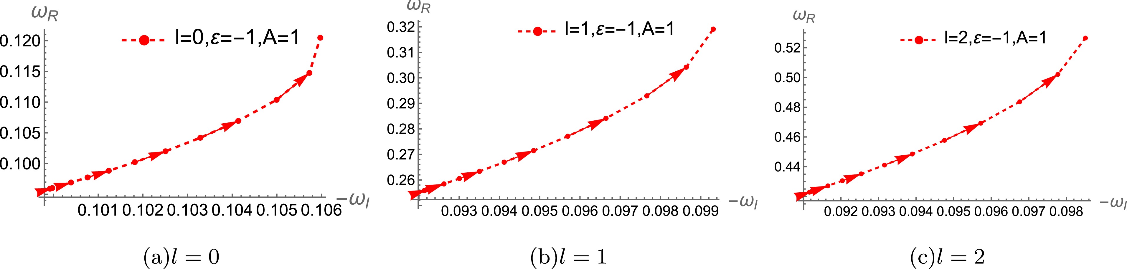

Figure 4.  (color online) Behaviors of real and imaginary parts of the 2nd branch black hole solution's QNMs under scalar perturbations for different l with $ M=1, L=1, \lambda=1 $. The arrows show the direction of the increase in black hole charge $ Q \in [0, 1.2] $.

Figure 5.  (color online) Behaviors of real and imaginary parts of the 1st branch black hole solution's QNMs under electromagnetic perturbations for different l with $ M=1, L=1, \lambda=1 $. The arrows show the direction of the increase in black hole charge $ Q \in [0, 1.1] $ in (a), (b), (c). $ Q \in [0, 1] $ in (d), (e), and (f).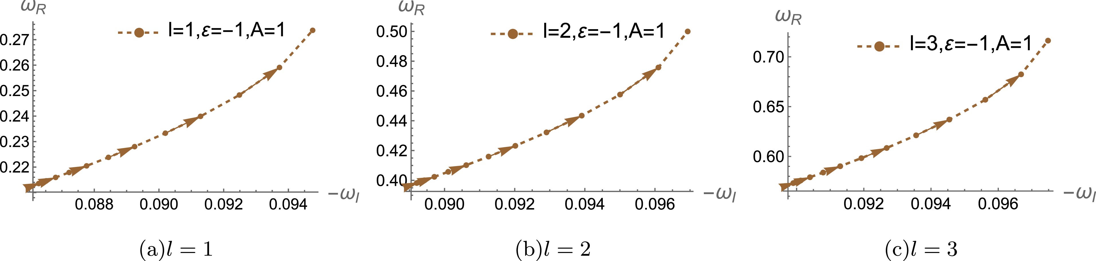

Figure 6.  (color online) Behaviors of real and imaginary parts of the 2nd branch black hole solution's QNMs under electromagnetic perturbations for different l with $ M=1, L=1, \lambda=1 $. The arrows show the direction of the increase in black hole charge $ Q \in [0, 1.2] $.

Figure 7.  (color online) Behaviors of real and imaginary parts of the 1st branch black hole solution's QNMs under gravitational perturbations for different l with $ M=1, L=1, \lambda=1 $. The arrows show the direction of the increase in black hole charge $ Q \in [0, 1.1] $ in (a), (b), (c). $ Q \in [0, 1] $ in (d), (e), (f).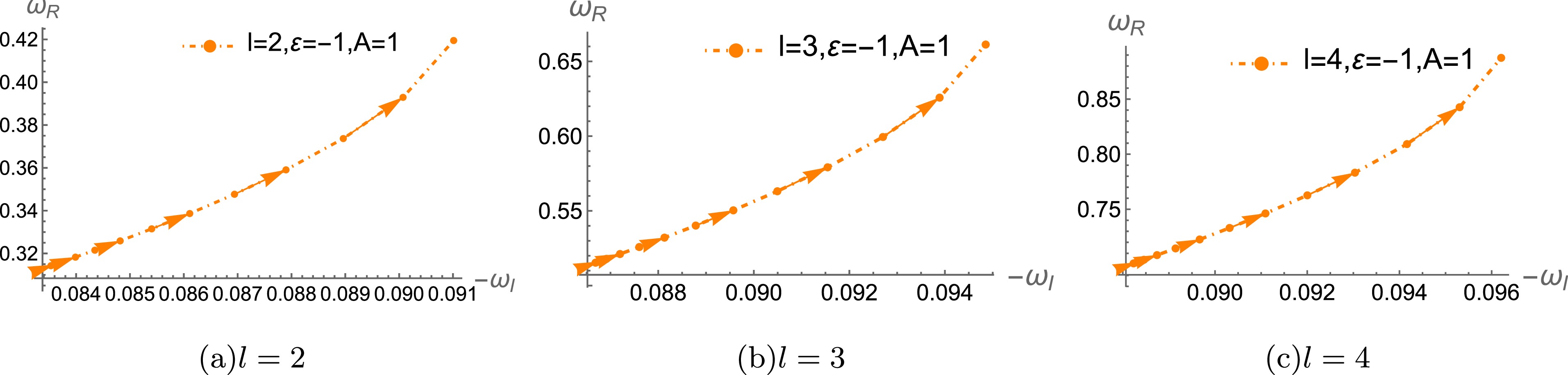

Figure 8.  (color online) Behaviors of real and imaginary parts of the 2nd branch black hole solution's QNMs under gravitational perturbations for different l with $ M=1, L=1, \lambda=1 $. The arrows show the direction of the increase in black hole charge $ Q \in [0, 1.2] $.

Let us begin by examining the imaginary part of the QNMs illustrated in Fig. 3, which show the behaviors of real and imaginary parts of the 1st branch black hole solution's QNMs under scalar perturbations. When we increase charge Q of the background configuration, we notice that the absolute value of the imaginary part of the quasinormal frequency $ |\omega_I| $ decreases for $ \varepsilon=1 $ (in Figs. 3(a),(b), (c)) and increases for $ \varepsilon=-1 $ (in Figs. 3(d),(e), (f)). Additionally, when the charge of the black hole Q and other parameters of the black hole are fixed, a larger value of angular momentum l results in a smaller $ |\omega_I| $. Specifically, for $ \varepsilon=1 $, the absolute value of the imaginary part decreases as the black hole charge increases. This indicates that the perturbations outside the black hole take a longer time to decay, meaning the perturbation remains active for an extended period before vanishing completely. From a holographic perspective, this implies that the dual system takes longer to return to equilibrium. For $ \varepsilon=-1 $, the behavior of $ |\omega_I| $ is indeed different, which suggests that the perturbations outside the black hole dissipate more rapidly as the black hole charge grows, contrary to the $ \varepsilon=1 $ case. This shows that the parameter ε has a significant influence on the stability and decay properties of the black hole.

Let us now examine the behavior of the real part of the quasinormal frequency $ |\omega_R| $, as depicted in the Fig. 3. For $ \varepsilon=1 $, as shown in Figs. 3(a),(b) (c), the real part of quasinormal frequency $ |\omega_R| $ increases as black hole charge Q increases. The arrows pointing from right to left indicate that when Q increases from $ 0 $ to $ 1 $, $ |\omega_R| $ gradually increases. This trend holds across different values of angular momentum l, meaning that as the black hole becomes more charged, the scalar perturbations gain energy, leading to higher oscillation frequencies. Furthermore, for fixed Q, the real part $ |\omega_R| $increases with increasing angular momentum l, implying that perturbations with larger angular momentum have more energy, regardless of charge Q. For $ \varepsilon=-1 $, the behavior is similar to that for $ \varepsilon=1 $.

We have discussed the QNM behaviors of scalar perturbations in the 1st branch black hole solution in detail. Similar results werefound for the second branch solutions as well as for electromagnetic and gravitational perturbations, as exhibited in Figs. 4−8. The behaviors of their QNMs align closely with the analysis presented earlier. Therefore, we do not repeat the detailed explanation here for these cases, as their characteristics exhibit similar trends across the different types of perturbations.

For black holes surrounded by a fluid of strings in four-dimensional Rastall gravity, we considered their scalar, electromagnetic, and gravitational perturbations. We applied the AIM to numerically compute the three perturbations and investigate the influence of black hole charge Q, angular momentum l, and model parameters ε on the quasinormal frequencies.

Specifically, for scalar perturbations and $ \epsilon = 1 $, we found that the absolute value of the imaginary part $ |\omega_I| $ decreases with increasing Q, indicating that the perturbations decay more slowly as the charge grows. Conversely, for $ \epsilon = -1 $, $ |\omega_I| $ increases with Q, suggesting that the perturbations dissipate more quickly. For the real part of quasinormal frequency $ |\omega_R| $, we observed a general trend of increasing frequency with both increasing black hole charge Q and angular momentum l. This indicates that the perturbations gain energy as the black hole becomes more charged or as the angular momentum of the perturbation increases, leading to higher oscillation frequencies. Importantly, these behaviors were consistent across both branches of black hole solutions and for all types of perturbations studied—scalar, electromagnetic, and gravitational fields.

Overall, our study emphasizes the intricate relationship between black hole parameters and the behavior of QNMs, offering insights into the stability and dynamics of black holes in the context of Rastall gravity. Future research could further explore the implications of these results for holographic dualities and the broader implications for black hole thermodynamics.

We would like to thank Nan Li for his selfless assistance.