Noncommutativity and its role in constant-roll inflation models with non-minimal coupling constrained by swampland conjectures

The fascination with understanding the genesis and evolution of the cosmos has endured since the dawn of scientific inquiry. However, we must acknowledge the stark disparity between our human scale of comprehension, limited by our dimensional constraints, and the vastness of cosmic dimensions. This vast chasm and our inherent limitations have necessitated the adoption of diverse approaches and tools to study the universe, all of which are fundamentally grounded in the principles of analogy and inference. The outcome is a plethora of theories, each meriting contemplation, ranging from Einstein's preference for a static universe to theories such as parallel universes, string theory, and the inflation hypothesis. These theories, while intriguing, cannot be definitively accepted or rejected owing to inherent flaws in each model. However, it appears that the inflation hypothesis is currently in the spotlight as it aligns with experimental data and our current understanding of the universe. This hypothesis is supported by experimental evidence such as the Hubble expansion of the universe and its ability to address several standard cosmological problems such as flatness and monopole issues. One of the main motivations for studying the early universe is to explain cosmic observations, such as large-scale structures and the temperature anisotropy of the cosmic microwave background (CMB) radiation. These observations suggest that the universe underwent a period of accelerated expansion, known as inflation. This solved several standard cosmological problems, such as the flatness and monopole problems. The simplest models of inflation are based on a scalar field ϕ that drives the dynamics of the expansion [1−4]. Einstein's theory of general relativity is one of the most outstanding achievements in physics, and it provides the foundation for modern cosmology. However, an open question remains: is general relativity a complete theory, or should it be modified at some level? Many efforts have been made to explore this possibility, and researchers have proposed various modifications to the theory of gravity from different perspectives. One of these approaches is Snyder's theory [5, 6], which introduces noncommutative (NC) space-time coordinates and modifies the renormalizability of quantum field theory. This theory also has implications for gravity as it introduces a short length cut-off and an NC parameter that becomes significant at the Planck scale [7−24].

The concepts of noncommutativity and deformed phase space have been extensively researched in the fields of gravity and cosmology over the last few decades, and they have the potential to transform our understanding of the universe. These concepts originate from quantum mechanics and quantum field theory, and they have significant implications for our cosmological knowledge. Noncommutativity refers to a property of certain mathematical operations in which the order of the operations matters, whereas deformed phase space is a theoretical framework for describing quantum systems. In these scenarios, the phase space (a mathematical space in which all the possible states of a system are represented) is modified or distorted in some form. This can result in new and intriguing behaviors for quantum systems, which can have important consequences for our understanding of gravity and the universe. These studies can possibly reveal new aspects of the nature of space and time, the dynamics of quantum systems, and the large-scale structure of the universe. For instance, noncommutativity has been applied to propose models of quantum gravity that attempt to unify the theories of quantum mechanics and general relativity. Similarly, deformed phase space scenarios have been employed to investigate the early universe and the nature of dark energy, among other topics. In recent decades, researchers have studied the effects of noncommutativity and deformed phase space scenarios on gravity and cosmology. These effects can also have observable consequences for the CMB spectrum as they can induce corrections to the primordial power spectrum and the spectral index [25−32]. The effects of the NC parameter on inflation, power-law inflation, and the CMB have been investigated using various models [33−38]. Recently, researchers have explored the impact of the NC parameter on the swampland conjectures, which are criteria that constrain the effective field theories that can be consistently coupled to quantum gravity, in the context of constant-roll inflation [39]. Constant-roll inflation is another approach to studying the early universe; it is an alternative to the conventional slow-roll approximation. In constant-roll inflation, the scalar field rolls down its potential with a constant rate, which leads to exact solutions of the inflationary equations. Moreover, some classes of constant-roll inflation models can be compatible with the observational data and produce realistic values for the inflationary observables, such as the scalar spectral index and the tensor-to-scalar ratio. Constant-roll inflation can also be generalized and combined with other models and theories, such as $ f(R) $ gravity, $ f(R, T) $ gravity, and teleparallel $ f(T) $ gravity, and the results can be compared and contrasted [40−50].

Swampland conjectures are criteria that aim to distinguish the effective field theories that can be consistently embedded in quantum gravity from those that cannot. These conjectures have been applied to study various cosmological concepts, such as inflation and the physics of black holes, and have yielded interesting results. Recently, new conjectures have been added to the swampland program to address some of the problems and inconsistencies that different models faced with the observational data. These approaches have been used to test the validity and viability of string theory, which is a leading candidate for a quantum theory of gravity. It would be intriguing to use such a framework to study the theories of inflation and cosmology from the perspective of string theory. For more studies on the applications of various swampland conjectures related to the physics of black holes, thermodynamics, cosmological inflation, etc., please refer to [51−83, 85−105].

Noncommutativity phase space is a concept that modifies the usual relations between the position and momentum variables of a physical system. In an NC phase space, the position and momentum variables do not have definite values, but they have uncertainties that depend on some constant parameters. These parameters are expected to be relevant at the Planck scale, where quantum gravity effects become important. Noncommutativity phase space has implications for various physical phenomena, such as the harmonic oscillator, hydrogen atom, Landau levels, Casimir effect, and CMB spectrum. It also affects the stability and renormalizability of some quantum field and higher derivative theories. In this paper, we aim to investigate four concepts: constant-roll inflation, NC parameter, non-minimal coupling (NMC), and swampland conjectures. We consider the constant-roll inflation scenario for the NMC field with the NC parameter and obtain exact solutions for the potential and other cosmological quantities. Researchers have explored various forms of coupling such as $ f = 1+\xi \phi $ with $ |\xi| = 0.1 $ and N = 60. In this paper, we want to select three different types of NMC functions: exponential, power-law, and logarithmic. We examine the compatibility or incompatibility of these functions with the NC parameter and swampland conjectures, which are criteria that constrain the effective field theories that can be consistently coupled to quantum gravity.

The remainder of this paper is organized as follows. In section II, we introduce the swampland program and explain the motivation for using the refined de Sitter (dS) swampland conjecture (RDSSC). In section III, we study the non-minimal coupling and noncommutativity effects in cosmological theories. We also discuss how these concepts motivate us to study the combination of NMC, RDSSC, NC, and constant-roll inflation. In Section IV, we analyze the constant-roll inflation in the presence of the NC parameter for the non-minimal coupling field and obtain the exact solutions. In section V, we test the compatibility of these concepts by introducing three different NMC functions. We also plot some figures to determine the allowed range for each case. We calculate the values of the scalar spectral index and the tensor to scalar ratio for two different potentials, and we compare them with the observational data from Planck 2018. We also determine the range of the free parameters (a; b; q) of the further refining de Sitter swampland conjecture (FRDSSC) that make the model consistent with the conjecture. Finally, we summarize the results in section VI.

The swampland program is a recent proposal to test string theory and its effective theories related to quantum gravity. String theory is one of the most prominent candidates for the theory of everything, and it has many implications for cosmology. The literature contains a rich and diverse collection of ideas and models that explore the cosmic aspects of string theory. [51−83, 85−105]. One of the intriguing features of string theory is that it has many possible vacua, typically of the order of $ ({\cal{O}}10^{500}) $, which form the landscape of string theory. A natural question that arises is which of these vacua correspond to effective low-energy theories that are consistent with string theory. This motivates the swampland program, which consists of many conjectures, such as the weak gravity conjecture, distance conjecture, and RDSSC. These conjectures aim to distinguish the effective theories that belong to the landscape from those that do not. The latter are called the swampland, and they occupy a larger region than the landscape. The swampland program uses various field-theoretical UV completion criteria derived from string theory, known as swampland conjectures, to classify different types of effective theories and determine whether they are in the swampland [51−105].

String theory is widely accepted as a theory that describes quantum gravity. Therefore, effective low-energy theories that are consistent with string theory are also compatible with quantum gravity, which can aid us in solving this big question that has puzzled researchers for years. The swampland program is a recent proposal to test string theory and its effective theories using various conjectures, such as the completeness conjecture [106], cobordism conjecture [107], distance conjecture, and RDSSC. These conjectures have many implications for cosmology, and much research has been conducted in this area. The RDSSC states that it is impossible to have dS vacua in string theory [108, 109]. However, note that some schemes, such as the KKLT construction [110], claim to produce dS vacua in string theory. The swampland program and its various conjectures have been widely and rapidly applied to different fields, such as inflation, black hole physics, and string theory. This program has also provided solutions to some problems and concepts that were incompatible with observational data. However, some theories have faced contradictions, which have been resolved by modifying or introducing new conjectures. One of the most significant challenges for the swampland program is the connection to the AdS/CFT correspondence [51−83, 85−105]. The swampland program can offer valuable insights into theoretical physics, but the crucial point is the fast and comprehensive development of this program in the context of physics and its consistency with observational data in conjunction with various approaches. It also raises questions about whether the swampland program can be a new revolution for string theory, whether it can become a complete theory, and whether it can be used in the fundamental concepts of theoretical physics. Many other questions can always attract curious minds. The swampland conjectures can also pose significant challenges to each of these possibilities. The swampland criteria have interesting implications for cosmology in the context of different models, such as single-field inflation [51, 55, 60, 61, 65, 67, 69, 71, 72, 74, 76, 79, 81, 83]. However, the observational data of the cosmological parameters show that single-field inflation is inconsistent with these conjectures [109]. Many attempts have been made to solve this problem, and some of them have been successful [111−113]. However, studies show that if the cosmological background of single-field inflation is not based on general relativity, these inflation scenarios can still be compatible with the swampland criteria [114−117]. Additionally, research has demonstrated that multi-field scenarios, even those based on general relativity, are consistent with the swampland conjectures [118]. Moreover, the warm inflation scenario, in both general relativity and non-general relativity frameworks, is fully compatible with the swampland conjectures [119, 120]. Many new conjectures have been added to the swampland program, each of which aims to extend this emerging concept or solve the problems that occur in inflationary cosmology. One of the most important ones is the trans-Planckian censorship conjecture (TCC) [ 121]. All these concepts motivate us to study the swampland conjectures from the perspective of NMC inflation scenarios in noncommutative phase space and to discuss the compatibility of this type of inflation scenario with string theory and quantum gravity. Therefore, we first explain the theory underlying the NMC inflation scenario. Subsequently, we reformulate this theory in the noncommutative phase space. Next, we investigate the cosmological consequences of this inflation scenario by applying the RDSSC and FRDSSC. We expect to obtain exciting results from the interplay of the swampland program, noncommutativity, and the NMC inflation scenario.

We introduce the general equations that describe the connections among the specific exact solutions that can be explicitly integrated for the cosmological models that involve a scalar field that is non-minimally coupled to gravity. Thus, we consider an action as [122−125],

where $ {\cal{R}} $ is the Ricci scalar, which is a measure of the curvature of the space-time. The space-time metric $ g_{\mu\nu} $ determines the distance between events and can be selected to have a specific form depending on the symmetry and boundary conditions of the problem. One of the most common choices is the Friedmann-Lemaître-Robertson-Walker (FLRW) metric, which assumes that the universe is homogeneous and isotropic, meaning that it appears the same at every point and in every direction. The FLRW metric can be expressed as ${\rm d}s^{2} = -{\rm d}t^{2}+a(t)^{2} ({\rm d}x^{2}+ $${\rm d}y^{2}+{\rm d}z^{2})$, where t is the cosmic time, x, y, and z are the spatial coordinates, and $ a(t) $ is the scale factor, which describes the change in the size of the universe with time. Using the FLRW metric and the scalar-tensor Lagrangian, we can obtain the action for the system, which is the integral of the Lagrangian over space and time. The action is a useful quantity to derive the equations of motion for the fields using the principle of least action. The action for the scalar-tensor theory in a FLRW background can be written as [122−125],

where the dot denotes the derivative with respect to the cosmic time. This action shows the coupling of the scalar field ϕ and scale factor a through the functions $ f(\phi) $ and $ V(\phi) $ and their effect on the evolution of the universe. We obtain this solution by varying the scale factor $ a(t) $. We can avoid the variation by using Noether's symmetry, but we will not discuss the changes caused by this symmetry in this article. The first challenge that we encounter in this article is to study the NMC field inflation in noncommutative phase space (NC). We will also examine the swampland conjecture in this context. We note that the NC effects at the classical and quantum levels in the cosmological system, as well as the UV/IR mixing for studying physical phenomena at different scales, provide us fascinating results from the perspective of quantum field theories [126−131]. The features of the NC model motivate us to investigate new and unknown phenomena in cosmology. Over the last decade, the applications and consequences of NC cosmology have been studied. For example, the gravitational collapse of a scalar field has been studied with special care. We consider a specific canonical noncommutativity and make a suitable deformation in the classical phase space. We use the deformed Poisson bracket between the canonical conjugate momenta, where we set $ \hbar = c = 1 $. Using this information, we can determine the NC parameter θ, which is crucial in investigating the point-like Lagrangian for the cosmology model and constant-roll condition [126−132],

The NC parameter θ is crucial for testing the NMC of the Lagrangian according to the swampland conjecture. An interesting point from the above equation is that noncommutativity on the momenta modifies the scalar field and scale factor. However, noncommutativity on the field and scale factor affects only the case of a non-vanishing potential. The noncommutativity parameter is introduced to modify the phase space of the inflationary model. This modification enables new dynamics that are not present in commutative models. The specific choice of $ \phi^3 $ is motivated by the desire to capture interesting and novel behaviors in the inflationary phase. We can propose a canonical deformation between momenta in a spatially flat FLRW universe. While the Friedmann equation (Hamiltonian constraint) remains unaffected, the Friedmann acceleration equation (and thus the Klein-Gordon equation) is modified by an extra term linear in the noncommutativity parameter. This extra term behaves as the sole explicit pressure, which implies a period of accelerated expansion of the universe under the right circumstances. Without the scalar field potential, the NC model predicts an inflationary phase for small negative values of the NC parameter. This contrasts with the commutative case, where the scale factor always decelerates. The period of accelerated expansion is smoothly replaced by an appropriate deceleration phase, providing an interesting model for the graceful exit problem in inflationary models. Additionally, note that some resemblance exists between the evolution equation of the scale factor in their NC model and that of the Starobinsky inflationary model. This resemblance suggests that the NC model can be a suitable scenario for successful kinetic inflation and can provide a graceful exit from inflation. The choice of the noncommutativity parameter involving $ \phi^3 $ enables the model to capture new dynamics and solve the horizon problem while providing a mechanism for inflation and graceful exit. This makes the noncommutative inflationary model a promising framework for understanding the dynamics of the early universe. Based on these explanations, we will derive the constant-roll inflation considering the NMC of the Lagrangian with NC phase space. Thereafter, we will apply the swampland conjectures and examine the impact of each of these factors. We will also obtain the relation between the above-mentioned concepts. We consider a generalized forms of coupling such as $ f = 1+\xi F(\phi) $ with $ |\xi| = 0.1 $ and we select three different types of NMC functions: exponential $ F(\phi) = \exp(\phi) $, power-law, $ F(\phi) = (\phi)^{n} $, and logarithmic $ F(\phi) = \log(\phi) $.

This section takes advantage of Hamiltonian formalism and examines the constant-roll inflation from the NMC concerning Eq. (2). Therefore, according to Eq. (2), the corresponding Hamiltonian for the model is calculated as

where $ P_{a} $, $ P_{\phi} $, and $ f(\phi) $ are momenta conjugates of scale factor, momenta conjugates of the scalar field, and NMC, respectively. As mentioned in the text, the coupling $ f(\phi) $ plays a significant role; therefore, we will explain the properties of different couplings in the present theory. The equation motions corresponding to the coordinates of the phase space $ a, \phi, P_{a} $, and $ P_{\phi} $ concerning the Hamiltonian Eq. (4) can be easily calculated. Therefore, according to the Hamilton in Eqs. (4) and (3), we can obtain $ \dot{a} = \{a, {\cal{H}}\} $, $ \dot{\phi} = \{\phi, {\cal{H}}\} $, $ \dot{P}_{a} = \{P_{a}, {\cal{H}}\} $, $\dot{P}_{\phi} = \{P_{\phi}, {\cal{H}}\},$ and $ \dot{P}_{f} = \{P_{f}, {\cal{H}}\} $, which are given in Appendix A. For the coupling f, which is a function of the scalar field ϕ, we define a conjugate as $ P_{f} $, where we have $ \{f, P_{f}\} = 1 $ and $ \{f', P_{f'}\} = 1 $. We also use the relationships between the parameter and their conjugates such as $ \{a, P_{a}\} = 1 $ and $ \{\phi, P_{\phi}\} = 1 $. Here, we also show the usual commutative equations of motion, which are obtained by setting $ \theta\rightarrow 0 $:

and

According to all the above concepts and relations, the equations of motion in the NC framework are calculated as follows:

We assume that $ 8\pi G = 1 $. By using some equations in Appendix A, we can obtain Eqs. (7) and (8), viz by squaring both sides of Eq. (61) and substituting Eq. (64) into Eq. (62), we obtain the Hamiltonian constraints, i.e., Eq. (7). Additionally, by taking the time derivative of Eq. (61) and using Eqs. (62), (63), (64), and (65), we obtain Eq. (8). As mentioned in the text, if we set the parameter θ to zero, the equations reduce to the standard ones in the literature. The pressure and energy density are denoted by $p_{\rm tot}$ and $\rho_{\rm tot}$ in the above equations. The equations of motion depend on the parameter θ, as shown in the above equations. We also maintain the values of θ to lower order because it has a shorter length than other parameters. We also consider the case of the noncommutative parameter $ \theta = 0 $, which leads to the conventional equations of motion. By using Eqs. (7) and (8) and the conditions, we calculate the constant-roll inflation for the non-minimally coupled field with the parameter θ. In this case, we obtain the exact values for the Hubble parameter, the potential, and other cosmological quantities. In the constant-roll studies, we also consider the assumptions mentioned below. Therefore, based on the equations of motion derived for the model with the NC parameter θ, we obtain the following results:

Given the relationship between the scale factor and Hubble parameter in the form $ H\equiv \dfrac{\dot{a}}{a} $, the above equation is written in the following form:

and by placing a very important relation, i.e., $\dot{H} = \dfrac{{\rm d}H}{{\rm d}\phi}\dot{\phi}$ in Eq. (10), we obtain

to examine the constant-roll condition of the mentioned inflation model, we must use the first derivative of the scalar field in Eq. (11) with respect to time. Therefore, the above equation is calculated using

Now, we benefit from the well-known condition of constant-roll, which is expressed as $ \ddot{\phi}-(3+\alpha)H\dot{\phi} $. In this case, by placing this condition in Eq. (12), we can calculate

To calculate the Hubble parameter accurately, we first assume that the parameter θ is zero. Thus, we have

and by solving Eq. (14), we can calculate

The above equation is a standard solution for the Hubble parameter in which the effects of the parameter θ are not observed in this structure. However, to obtain a specific solution for the parameter θ, we take the solution of the Hubble parameter in Eqs. (15) and (13). Therefore, we consider a general ansatz for such an anisotropy structure of inflation, which is obtained using

By placing ansatz in Eq. (13) and performing a series of simple manipulations, values of the parameter λ can be obtained. Therefore, we can obtain specific solutions for the Hubble parameter and other quantities such as potential by considering a series of boundary conditions. Having these exact solutions in the continuation of the article, we can obtain a special relationship between such an inflation model in the presence of the parameter θ concerning coupling $ f(\phi) $ and swampland conjectures. Therefore, we will first calculate the specific answers according to the boundary conditions.

We start this subsection by considering a boundary condition of $ c_{1} = c_{2} = \dfrac{M}{2} $ for Eq. (16), which provides us two different values for the parameter λ. We select the positive value of λ. Thereafter, we obtain the exact solution of the Hubble parameter with the effects of various parameters, particularly the parameter θ. Using the exact solution of the Hubble parameter $ (H) $, we also compute the potential $ (V) $ and the quantity of $ \dot{\phi} $. We have provided the solution in Appendix B. In the continuation of calculations, by obtaining the quantity ϕ in terms of time t, the Hubble parameter can be easily calculated in terms of time. Additionally, according to the relationship between the Hubble parameter and scale factor mentioned as $ H = \dfrac{\dot{a}}{a} $, we can easily calculate the scale factor. Now, we consider another boundary condition.

We start this subsection by considering a different boundary condition of $ c_{1} = \dfrac{M}{2} $ and $ c_{2} = -\dfrac{M}{2} $. As in the previous subsection, we obtain two different values for the cosmological quantities H, $ V(\phi) $, and $ \dot{\phi} $. We select the positive values, but we can also obtain the negative values through an iterative process. Based on the explanations, we compute the Hubble parameter, the potential $ V(\phi) $, and $ \dot{\phi} $, which are given in Appendix B. We apply the swampland conjectures to the potentials obtained from different boundary conditions and plot the results. Our aim is to investigate the relations of the swampland conjecture to the constant-roll inflation with the NC parameter θ and different types of NMCs, such as exponential, logarithmic, and power-law. The figures below show the logarithmic coupling on the left, the exponential coupling in the middle, and the power-law coupling on the right, for different swampland components and potentials. We will explain the relationship between these concepts in detail. Another important point is that we assume the constant parameter α to be in the range of $ -3<\alpha<3 $. The figures also show that for the exponential coupling $ F(\phi) = \exp(\phi) $, the logarithmic coupling $ F(\phi) = \log(\phi) $, the power-law coupling $ F(\phi) = (\phi)^{n} $ gives acceptable results for $ \theta>0 $.

We study the effects of NC phase space and constant-roll condition on the RDSSC using different types of coupling $ f(\phi) $, such as power-law, exponential, and logarithmic. We present the results for each case in detail with some figures. In this section, we apply the refined swampland conjectures to the exact solutions of the potential obtained from different boundary conditions. The swampland conjecture component depends on two critical parameters: the NC parameter θ and NMC $ f(\phi) $. These concepts can be tested against each other. We observe some interesting results from the interplay of RDSSC, NMC, the NC parameter, and constant-roll condition. We investigate the relation of each coupling to the swampland conjecture component with the NC parameter θ.

Here, we present the conjecture that improves the de Sitter swampland conjecture with more precision. We examine a 4D theory of a real scalar field interacting with gravity, where the scalar potential governs its behavior. The action of this theory has the following form [51, 55, 59, 61, 65, 67, 69, 71, 72, 74, 76, 79, 81, 83, 84]:

In this equation, $ M_{p} $, $ h_{ij} $, and $ R_{4} $ denote the Planck mass, field metric, and 4D Riemann curvature, respectively. The RDSSC imposes several constraints on the potential of the effective theory, as shown in the following equation [51, 55, 59, 61, 65, 67, 69, 71, 72, 74, 76, 79, 81, 83]:

where $ C_1 $ and $ C_2 $ are constants of order unity. According to Eqs. (22) and (18), we obtain

$ C_1 $ and $ C_2 $ can appear as coefficients in front of terms involving the potential and its derivative equations governing the inflationary dynamics in the context of the swampland conjectures. They are often defined as a parameter that encapsulates the constraints imposed by the swampland conjectures on the inflationary potential. These conjectures suggest that certain conditions must be satisfied for a theory to be consistent with a quantum gravity framework. They relate to affection the shape and steepness of the inflationary potential, ensuring that the model remains within the bounds set by the swampland conjectures. It aids in determining the viability of the inflationary model in a quantum gravity context.

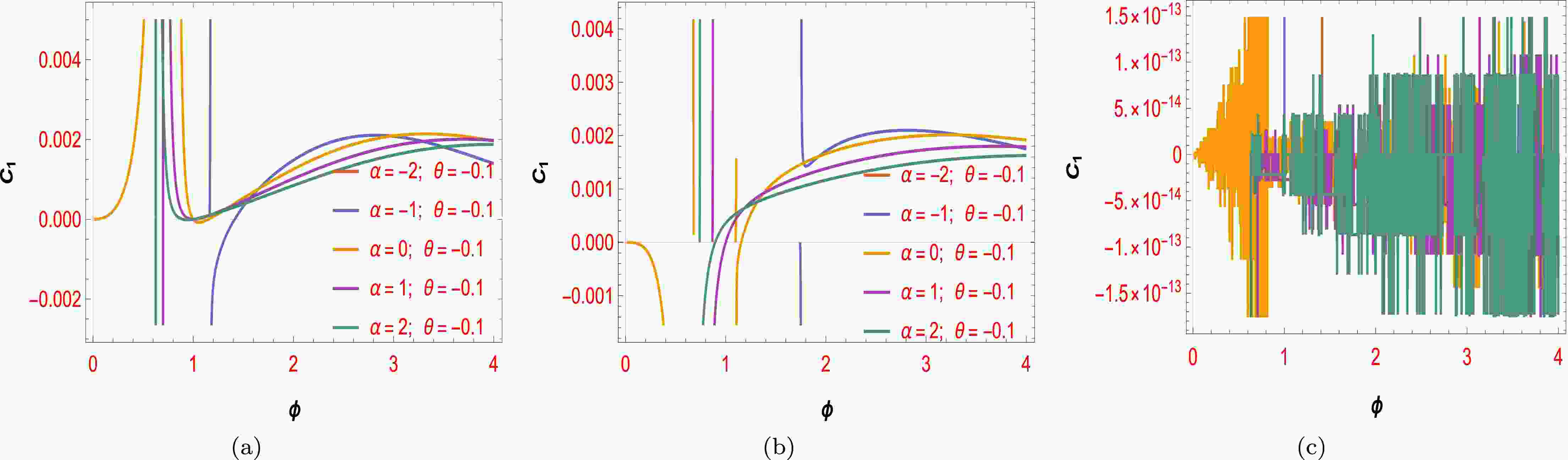
The following figures show the constraints of the swampland conjecture components, $ C_{1} $ and $ C_{2} $, derived from the potential of the constant-roll inflation with the NC parameter θ and NMC $ f(\phi) $. Fig. 1 and Fig. 3 show the constraint of component $ C_{1} $ for potential V according to the first boundary conditions of different NMCs. We consider three types of couplings: exponential, power-law, and logarithmic. Figs. 1(a), 1(b), and 1(c) show that none of these couplings have acceptable regions with respect to the dS swampland conjecture for $ \theta = -0.1 $. However, Figs. 3(a), 3(b), and 3(c) show that these couplings have acceptable ranges for the constraint of component $ C_{1} $ for $ \theta = +0.1 $. The literature reveals that the swampland conjecture components are always positive values of order one. The figures clearly show the constraints of each component for different values of the constant parameter $ -3<\alpha<3 $ and $ \theta = +0.1, -0.1 $. The results in Fig. 3 are more interesting and compatible than those in Fig. 1 for the conjecture components $ C_{1} $. Fig. 2 and Fig. 4 also plot the constraint of component $ C_{2} $ as a function of the scalar field ϕ for potentials V with different values of α according to the first boundary condition. These figures depict the constraints of each component for each coupling. The component $ C_{2} $ is also a positive value of order one. As shown in Fig. 4, the allowed values for each coupling are more consistent with the dS swampland conjecture than those for the potential in Fig. 2 and cover more acceptable general ranges. In summary, the solutions for Fig. 3 and Fig. 4 have more compatibility and acceptable ranges for the dS swampland conjectures. Another point to note is that each coupling has such solutions within a specific range of θ. We observe that, generally, the logarithmic, power-law, and exponential couplings in the range $ \theta<0 $ do not yield reasonable solutions.

Figure 1.  (color online) Plot of the variation in $C_{1}$ in terms of $\phi$ for logarithmic non-minimal coupling in (a), exponential non-minimal coupling in (b), and power-law non-minimal coupling in (c) with respect to the constant parameter $-3<\alpha<3$, ($\theta<0$) and potential $V_{1}(\phi)$ from case I.

Figure 2.  (color online) Plot of the variation in $C_{2}$ in terms of $\phi$ for logarithmic non-minimal coupling in (a), exponential non-minimal coupling in (b), and power-law non-minimal coupling in (c) with respect to the constant parameter $-3<\alpha<3$, ($\theta<0$) and potential $V_{1}(\phi)$ from case I.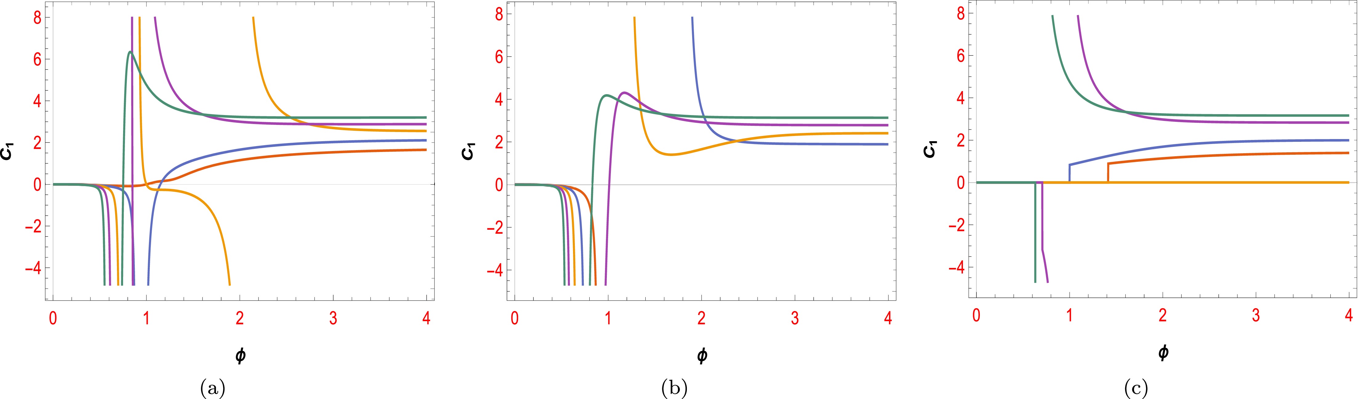

Figure 3.  (color online) Plot of the variation in $C_{1}$ in terms of $\phi$ for logarithmic non-minimal coupling in (a), exponential non-minimal coupling in (b), and power-law non-minimal coupling in (c) with respect to the constant parameter $-3<\alpha<3$, ($\theta>0$) and potential $V_{2}(\phi)$ from case I.

Figure 4.  (color online) Plot of the variation in $C_{2}$ in terms of $\phi$ for logarithmic non-minimal coupling in (a), exponential non-minimal coupling in (b), and power-law non-minimal coupling in (c) with respect to the constant parameter $-3<\alpha<3$, ($\theta>0$) and potential $V_{2}(\phi)$ from case I.

We obtain the constraints of the first component of the swampland conjecture as a function of the scalar field for the potential from the second boundary condition, based on the explanations we gave for Fig. 1 to Fig. 4 from the first boundary condition. We consider the different couplings and show constraints of the first component of the dS swampland $ C_{1} $ in Fig. 5 and Fig. 7. We also determine the constraints of the second component of the swampland $ C_{2} $ for the same structure in Fig. 6 and Fig. 8. The power-law coupling does not have acceptable ranges for the first component $ C_{1} $ for the potential in Fig. 5(c), unlike the other two couplings. Fig. 6 shows that the second component of the swampland for V from the second boundary condition has much more acceptable regions than $ C_{1} $ for all couplings. For V from the second boundary condition, the constraints of both components of the swampland are plotted as a function of ϕ in Fig. 7 and Fig. 8. They have more acceptable ranges than V from the first boundary condition in Fig. 5 and Fig. 6. The constraints are plotted for different values of the constant parameter $ -3<\alpha<3 $ and $ \theta = -0.1, 0.1 $ in all the figures. Generally, Fig. 1 and Fig. 2 from the first boundary condition and Fig. 5(c) for the power-law coupling from the second boundary condition do not have acceptable ranges for the dS swampland conjecture. However, $ \theta = 0.1 $ has a much more acceptable region than $ \theta = -0.1 $ and is more compatible with the dS swampland conjecture. Our study shows that the order of consistency of the couplings with the dS swampland conjecture is exponential NMC $ > $ logarithmic NMC $ > $ power-law NMC.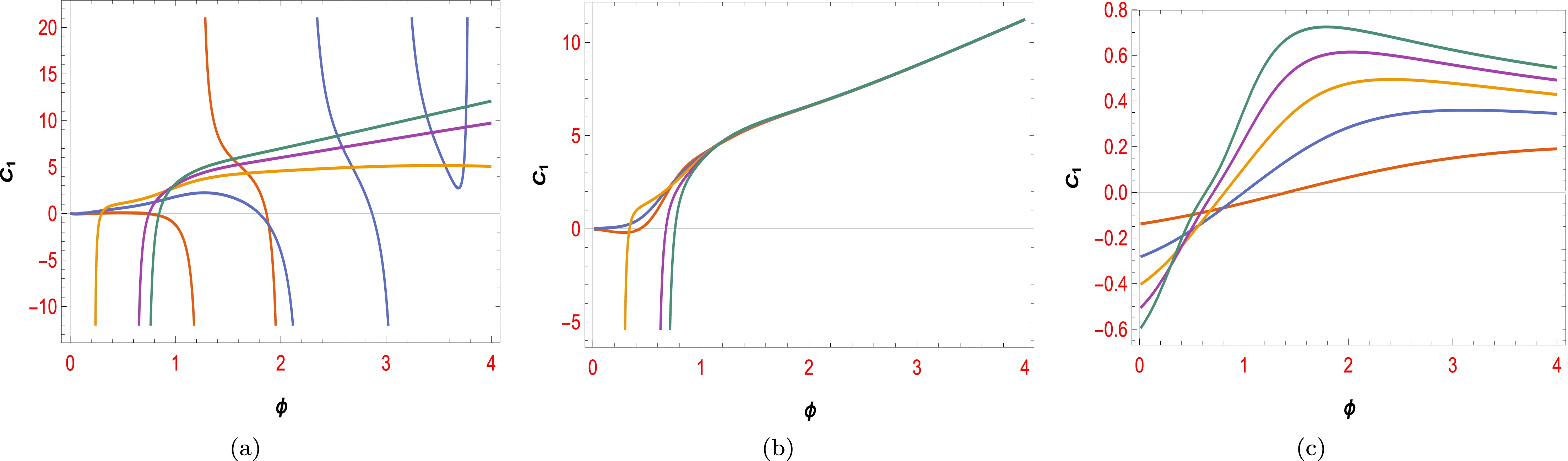

Figure 5.  (color online) Plot of the variation in $C_{1}$ in terms of $\phi$ for logarithmic non-minimal coupling (a), exponential non-minimal coupling in (b), and power-law non-minimal coupling in (c) with respect to the constant parameter $-3<\alpha<3$, ($\theta<0$) and potential $V_{1}(\phi)$ from case II.

Figure 6.  (color online) Plot of the variation in $C_{2}$ in terms of $\phi$ for logarithmic non-minimal coupling (a), exponential non-minimal coupling in (b), and power-law non-minimal coupling in (c) with respect to the constant parameter $-3<\alpha<3$, ($\theta<0$) and potential $V_{1}(\phi)$ from case II.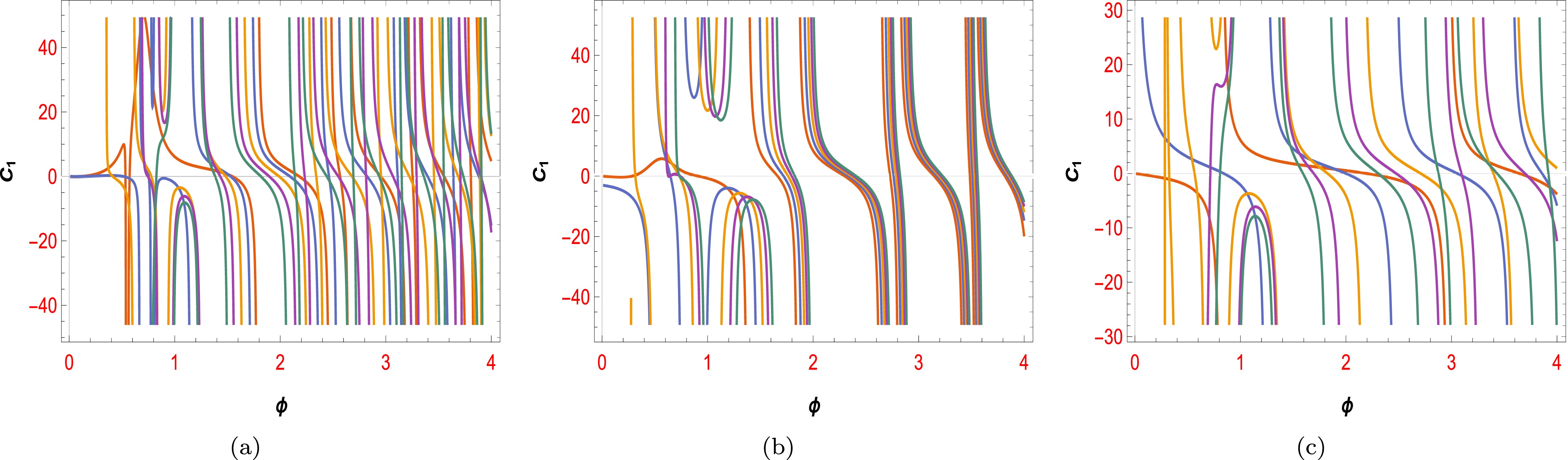

Figure 7.  (color online) Plot of the variation of $C_{1}$ in terms of $\phi$ for logarithmic non-minimal coupling in (a), exponential non-minimal coupling in (b), and power-law non-minimal coupling in (c) with respect to the constant parameter $-3<\alpha<3$, ($\theta>0$) and potential $V_{2}(\phi)$ from case II.

Figure 8.  (color online) Plot of the variation in $C_{2}$ in terms of $\phi$ for logarithmic non-minimal coupling in (a), exponential non-minimal coupling in (b), and power-law non-minimal coupling in (c) with respect to the constant parameter $-3<\alpha<3$, ($\theta>0$) and potential $V_{2}(\phi)$ from case II.

Using all the concepts discussed above, we will calculate some of the most important parameters of cosmology and discuss them. Therefore, we will consider the following parameters. We can calculate the slow-roll parameters of the model using

The prime symbol indicates the derivative with respect to the bilinear field ϕ. Inflation terminates when either $ \epsilon = 1 $ or $ \eta = 1 $. The number of e-folds is determined by

We can also introduce the spectral parameters, namely, the spectral index, its running, and the tensor-to-scalar ratio. These are defined as follows:

We can derive the tensor-to-scalar ratio by adding a single parameter tensor component to the ΛCDM model, which yields $ r_{0.002} < 0.10 $ (95% CL, Planck TT + lowE + lensing) [133−135]. This result agrees with the recent observations and also with $ r_{0.002} < 0.056 $ (95% CL, Planck TT, TE, EE + lowE + lensing + BK15) [135] and $ r_{0.002} < 0.064 $ (95% CL, Planck TT, TE, EE + lowE + lensing + BK15 and Virgo2016). Moreover, the Planck 2013 data analysis [133] provides the value of the Hubble constant as $ 67.36 \pm 0.54 $ km/s/Mpc⁻¹ from Planck TT, TE, EE + lowE + lensing. The running of the scalar spectral index in simple inflation models is very small and depends on the second-order of the slow-roll parameters: $ (dn_s/d\ln k) \approx -0.0045 \pm 0.0067 $ (68% CL) from Planck TT, TE, EE + lowE + lensing [135]. Furthermore, these significant parameters can be confirmed using the latest Planck data, which has a 68 percent error. In contrast, the $ n_s $ and r constraints are derived from the marginalized joint 68% and 95% CL regions of the Planck 2018 combined with BK14 + BAO data, i.e., $ n_s = 0.9649 \pm 0.0042 $ at 68% CL, r < 0.1 at 95% CL and from the recent BICEP2/Keck Array BK14 data $ r<0.056 $ at 95 % CL [135, 136]. The spectral index $ n_s $ measures the scale dependence of the primordial power spectrum of scalar perturbations. It is defined as $n_s - 1 = \dfrac{{\rm d} \ln P_s(k)}{{\rm d} \ln k}$, where $ P_s(k) $ is the power spectrum of scalar perturbations, and k is the wavenumber. In the context of inflation, $ n_s $ can be computed using the slow-roll parameters ϵ and η as shown in Eq. (22), where ϵ and η are also defined in Eq. (20). Additionally, V is the potential of the inflaton field, and $ V' $ and $ V'' $ are its first and second derivatives for the field, respectively. The tensor-to-scalar ratio r quantifies the relative contribution of tensor (gravitational wave) perturbations to scalar perturbations. It is given by $ r = \dfrac{P_t(k)}{P_s(k)} $, where $ P_t(k) $ is the power spectrum of tensor perturbations. In terms of the slow-roll parameter ϵ, r can be expressed as Eq. (22). The introduction of the noncommutativity parameter modifies the standard commutation relations between the coordinates or fields, which can affect the dynamics of the inflaton field and the resulting perturbations. Specifically, the NC parameter θ can introduce additional terms in the equations of motion, leading to modifications in the slow-roll parameters ϵ and η. For example, the modified Klein-Gordon equation in an NC space might include terms proportional to θ, altering the evolution of the inflaton field. Consequently, the expressions for $ n_s $ and r would also be modified to account for these additional terms. This can lead to deviations from the standard predictions of $ n_s $ and r, but in some regions, we have an acceptable range owing to some coupling as explained in this work. In constant-roll inflation, the rate of change of the inflaton field is constant, which differs from the slow-roll approximation where the field slowly rolls down its potential. The constant-roll condition is given by $ \ddot{\phi} = \beta H \dot{\phi} $, where β is a constant parameter. Because of this condition, the slow-roll parameters ϵ and η are not necessarily small, and their standard definitions might not apply. Instead, the spectral index $ n_s $ and tensor-to-scalar ratio r are computed using the modified dynamics of the inflaton field under the constant-roll condition. The spectral index in constant-roll inflation can be expressed as $ n_s = 1 + 2\beta - 2\epsilon $, where β is the constant-roll parameter, and ϵ is still defined as before but may not be small. The tensor-to-scalar ratio r in constant-roll inflation is similarly affected by the constant-roll parameter β and the modified dynamics of the inflaton field. These modifications ensure that the calculations of $ n_s $ and r are consistent with the underlying dynamics of the inflaton field in an NC phase space and under constant-roll conditions.

One of the main objectives of cosmology is to measure the parameters that describe the evolution and structure of the universe. Among these parameters, the tensor-to-scalar ratio r and scalar spectral index $ n_s $ are particularly important, as they can reveal information about the physics of the early universe and the mechanism of inflation. Inflation is a hypothetical period of exponential expansion that occurred shortly after the Big Bang and driven by a scalar field called the inflaton. The inflaton potential $ V(\phi) $ determines the dynamics and properties of inflation, such as the duration, energy scale, and generation of primordial perturbations. Therefore, by comparing the predictions of different inflationary models with the observational data, we can test the validity and compatibility of these models. In this section, we calculate and plot the spectral parameters, i.e., the spectral index $ n_s $ in terms of r for both cases using the potentials in Appendix B and Eqs. (20) and (22). These equations relate the spectral parameters to the inflaton potential and its derivatives, as well as the NMC function and its derivatives. We consider the free parameters of the models, such as $ \alpha = -1, 1 $ and $\theta = -0.1,\; 0.1$ that appear in the NMC function. We plot the $ (r-n_s) $ diagram for different values of these parameters and NMCs in Fig. 9 and Fig. 10. Fig. 9 shows the variations in the $ (r-n_s) $ for the first boundary condition with respect to the parameters α and θ. The effects of these mentioned concepts are clearly visible in the figures. They can change the shape and position of the $ (r-n_s) $ curve and make it cross the observational bounds. We also plot the same variations for the second case in Fig. 10. We observe that the NMC can also alter the predictions of this model and make it more or less compatible with the data. Subsequently, by selecting the best specific value for r and $ n_s $ for each case and considering power-law, logarithmic, and exponential NMC, we determine the compatibility of each model with another one of the most important conjectures of the swampland program. The swampland program is a research program that aims to identify the consistent theories of quantum gravity and distinguish them from the inconsistent ones. The swampland conjectures are criteria that any effective field theory must satisfy to be compatible with quantum gravity. One of these conjectures is the FRDSSC. In the next section, we test this conjecture for our inflationary model and observe the effects on NMC on the results.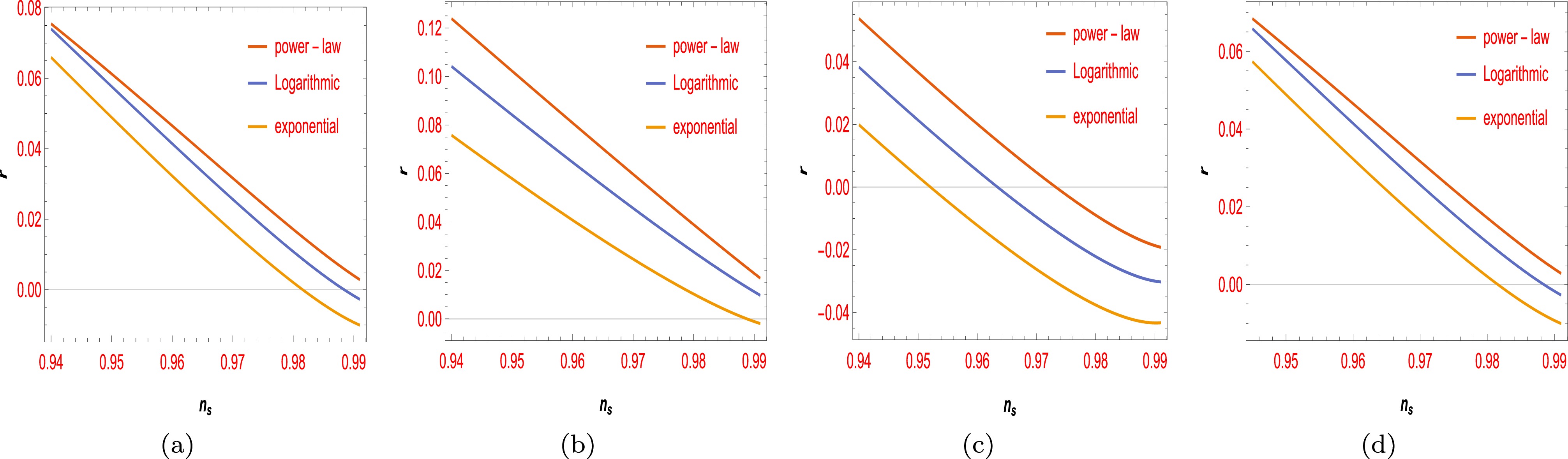

Figure 9.  (color online) The plot of the $(r-n_s)$ for power-law, logarithmic, and exponential non-minimal coupling with respect to the constant parameter $\alpha=-1, 1$ and $\theta<0$ in (a) and (b), and $\alpha=-1, 1$ and $\theta>0$ in (c) and (d) for case I.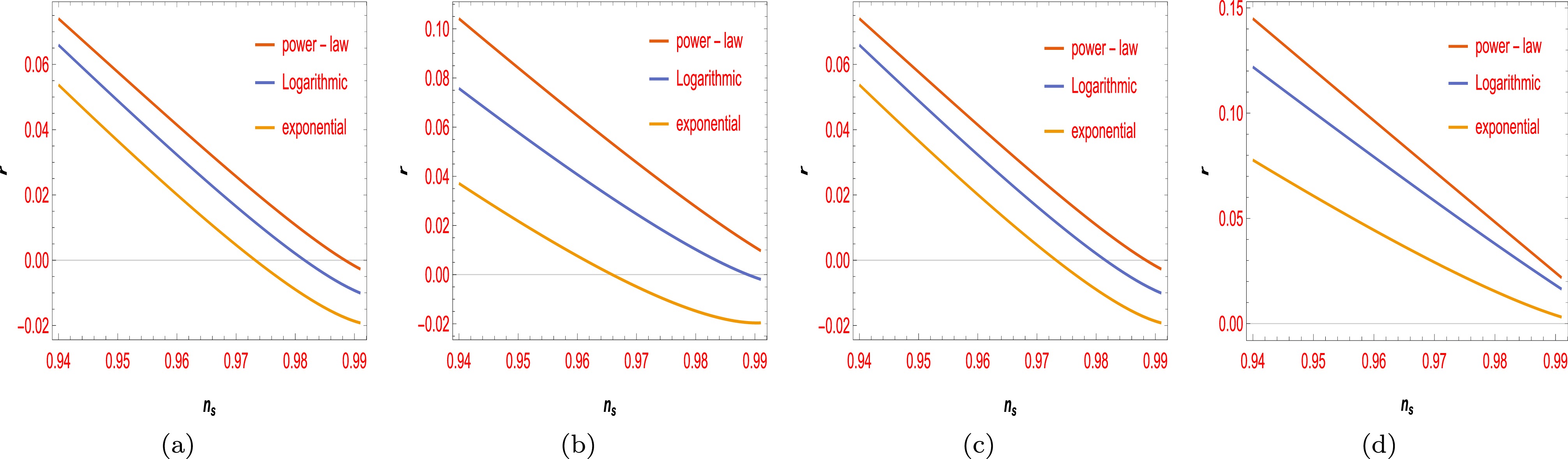

Figure 10.  (color online) The plot of the $(r-n_s)$ for power-law, logarithmic, and exponential non-minimal coupling with respect to the constant parameter $\alpha=-1, 1$ and $\theta<0$ in (a) and (b), and $\alpha=-1, 1$ and $\theta>0$ in (c) and (d) for case II.

We obtain and plot the important cosmological parameters $ (n_s-r) $ for second boundary condition with respect to Eqs. (20) and (22) for various NMCs considering the free parameters.

The expressions Eqs. (18) and (19) for the refined swampland conjecture are not very illuminating, as there is a lack of connection between these two criteria. They are unable to offer any information jointly based on their formulations. Hence, David Andriot and Christoph Roupec developed the preceding conjectures and proposed a new correlation termed the further refining de Sitter swampland conjecture (FRDSSC), which can furnish us with a comprehensive account and amalgamate the two prior equations [51, 55, 59, 61, 65, 67, 69, 71, 72, 74, 76, 79, 81, 83]:

Let $ a+b = 1 $, $ a,b>0 $, and $ q>2 $. The constants a, b, and q impose a constraint for this conjecture. The preceding conjecture can also be reformulated in terms of the slow-roll parameters, as shown below

In this paper, we want to challenge the models with the FRDSSC. The compatibility of the model with this new conjecture is achieved by adjusting the free parameters. For a scalar field potential, we define the following quantities:

where $V_{,} = {\rm d}V(\phi)/{\rm d}\phi$ and $V_{,,} = {\rm d}^{2}V(\phi)/{\rm d}\phi^{2}$. According to the explanations, we obtain

Additionally, when the slow-roll approximation is valid, each of the preceding equations can be reformulated in terms of two key cosmological parameters: the scalar spectral index and tensor-to-scalar ratio. Based on the arguments, we have presented

Next, we evaluate the model using the RDSSC and ascertain its compatibility and incompatibility. We note that if the model satisfies these conjectures, it will belong to the landscape rather than the swampland, which is somewhat compatible with quantum gravity.

In this section, we aim to check the compatibility of another conjecture of the swampland program with the model. Therefore, we study this consistency according to the above explanation by considering the potentials in two boundary conditions and with respect to r and $ n_s $, as well as each of the couplings. Thus, according to the V in the first boundary condition, the values of $ (n_s, r) $ are obtained as $(n_s = 0.964878,\;\;r = 0.0130472)$, $(n_s = 0.964872, r = 0.0236971)$, and $(n_s = 0.964862,\;\; r = 0.0337863)$ for each of the exponential, logarithmic, power law NMCs, respectively. In the following, according to the calculated values, we will check their compatibility with the FRDSSC and determine the range of compatibility for each model.

$ \bullet $ Exponential: $ n_s = 0.964878 $ $,\;$ $ r = 0.0130472 $

Here, according to the mentioned case for first boundary condition and with respect to Eqs. (29) and (30), we obtain

According to Eqs. (24), (29), and (30), we obtain

Considering a series of straightforward calculations, we can obtain

With the assumption $ q = 2.4 $, we will have

Therefore, if we consider $ a = 0.989231 $, b is calculated as

Therefore, this case is consistent with the FRDSSC. We can also satisfy the conjecture by manually adjusting the free parameters (a,b,q) of the FRDSSC, as we have performed in the previous section.

$ \bullet $ Logarithmic: $n_s = 0.964872,$ $ r = 0.0236971 $

Now, we can calculate for first boundary condition and logarithmic NMC considering Eqs. (29) and (30):

Therefore, with respect to Eqs. (24), (29), and (30), we can obtain

With a series of calculations, we obtain

By considering $ q = 2.4 $, we obtain

By selecting $ a = 0.997231 $,

Therefore, this case is consistent with the FRDSSC, and the free parameters (a, b, q) are satisfied.

$ \bullet $ Power law: $n_s = 0.964862,$ $ r = 0.0337863 $

Similar to the pervious part, for the first boundary condition and power law NMC with respect Eqs. (29) and (30), we obtain

with respect to Eqs. (24), (29), and (30), we can obtain

Additionally, we have

If we assume the $ (q = 2.4) $ in the above equation, then we will obtain

According to Eq. (44), by selecting a suitable value for the parameter $ a = 0.988921 $, we calculate another free parameter as follows:

Therefore, this case is also consistent with the FRDSSC, and the free parameters (a, b, q) are satisfied.

For V in the second boundary condition, $ (n_s, r) $ has been calculated as $(n_s = 0.964878,\; r = 0.0226542)$, ($n_s = 0.964872,\; r = 0.0316693)$, and $(n_s = 0.964862, r = 0.0391818)$ for the exponential, logarithmic, power law NMCs, respectively. We will fully study the compatibility of them with the FRDSSC and determine the range of compatibility for each model.

$ \bullet $ Exponential: $n_s = 0.964878,$ $ r = 0.0226542 $

Now, we can calculate for second boundary condition with respect to the exponential NMC considering Eqs. (29) and (30):

With respect to Eqs. (24), (29), and (30), we obtain

Therefore, we can obtain

We select $ q = 2.4 $ from Eq. (48). Thus,

By selecting $ a = 0.988632 $ from Eq. (49), we obtain

Here, $ V_2 $ with respect to the exponential NMC is also consistent with the FRDSSC, and the free parameters (a, b, q) are satisfied.

$ \bullet $ Logarithmic: $n_s = 0.964872,$ $ r = 0.0316693 $

Additionally, for the second boundary condition with respect to the logarithmic NMC considering Eqs. (29) and Eq. (30), we can obtain

With respect to Eqs. (24), (29), and (30), we will obtain

Therefore, we have

We select $ q = 2.4 $:

From Eq. (54) and by selecting $ a = 0.99123 $, we obtain

Thus, $ V_2 $ with respect to the logarithmic NMC is also consistent with the FRDSSC, and the free parameters (a, b, q) are satisfied.

$ \bullet $ Power law: $n_s = 0.964862,$ $ r = 0.0391818 $

We can obtain for second boundary condition with respect to the power law NMC considering Eqs. (29) and (30):

With respect to Eqs. (24), (29), and (30), we obtain

Also, we have,

We consider $ q = 2.4 $. Therefore, we obtain

By selecting $ a = 0.992469 $, we can calculate

Thus, $ V_2 $ with respect to the power law NMC is also consistent with the FRDSSC, and the free parameters (a, b, q) are valid.

In this paper, we study constant-roll inflation and the swampland conjectures for the non-minimal coupling field in the perspective of noncommutative phase space. Using the Hamiltonian formalism, we obtain the solutions of constant-roll inflation according to the noncommutative parameter and non-minimal coupling field of the Lagrangian. We consider three different types of couplings: power-law, exponential, and logarithmic. Subsequently, by plotting some figures, we study the effects of these coupling in constant-roll inflation with noncommutative parameters. We identify and specify the permissible regions of each case about the swampland conjectures and determine the best model. We find that the exponential logarithmic and power-law coupling with $ \theta>0 $ agree with the dS swampland conjecture. These couplings yield similar results in both cases, some compatible and some incompatible with the dS swampland conjectures. Moreover, $ \theta>0 $ is more compatible than $ \theta<0 $, and the consistency value in the second boundary condition is much higher than that in the first. The order of better compatibility of couplings with the swampland conjecture is ranked as follows: exponential non-minimal coupling, logarithmic non-minimal coupling, power-law non-minimal coupling. For each type of coupling, we calculate the values of the scalar spectral index $ n_s $ and the tensor-to-scalar ratio r for two different potentials. We compare them with the observational data from Planck 2018. We also determine the range of the free parameters $ (a,b,q) $ of the further refining de Sitter swampland conjecture (FRDSSC) that makes the model consistent with the conjecture. We find that the model satisfies the FRDSSC for all types of couplings and both potentials, with some constraints on the parameters.

In conclusion, we have shown that constant-roll inflation with noncommutative parameters and non-minimal coupling fields can provide viable models of inflation that are compatible with the swampland conjectures and observational data. We also explore the effects of different types of couplings and potentials on the inflationary dynamics and swampland criteria. We find that the exponential and logarithmic couplings are more favorable than the power-law coupling in terms of satisfying the dS swampland conjecture. Additinoally, the potential with $ \theta>0 $ is more consistent than the potential with $ \theta<0 $ in terms of swampland conjectures. We also test the model against the FRDSSC and find that it is satisfied for all cases, with some bounds on the parameters $ (a,b,q) $. Some questions arise from our study that we leave them for future research. 1) How does the noncommutative parameter affect the reheating process and the generation of primordial perturbations? 2) How does the non-minimal coupling field affect the quantum corrections and the stability of the inflationary solutions? 3) How can we embed our model in a consistent UV completion, such as string theory or quantum gravity? 4) How can we test our model with future observations, such as the BICEP3 experiment or the Planck?

We have some parameters as a, ϕ, f, and $ f' $, and their corresponding momenta are $ P_a $, $ P_\phi $, $ P_f $, and $ P_{f'} $. The Hamiltonian is given by Eq. (4). Using the given relations between the parameters and their conjugates, we can calculate the Poisson brackets. To determine the specific values of these Poisson brackets, we must take the partial derivatives of the Hamiltonian with respect to the variables:

The solutions of the Hubble parameter $ (H) $, potential $ (V) $, and quantity of $ \dot{\phi} $ are calculated as

Additinally,

and

The Hubble parameter, potential $ V(\phi) $, and $ \dot{\phi} $ for case II are given by

Additionally,

and