Accretion of Vlasov gas onto a black hole in the Kalb–Ramond field

The accretion of matter by a black hole (BH) is a fundamental concept in astrophysical studies, offering insights into the origins of high-energy X-rays and γ-ray bursts. Several studies have pioneered the research in this field [1−3]. Furthermore, Bondi used Newtonian dynamics to investigate the steady spherical accretion of a gas at rest at infinity onto a star [4]. Michel later generalized Bondi’s work to general relativity, focusing on the accretion of a perfect fluid onto a Schwarzschild BH [5]. Subsequent research has examined various aspects of BH accretion models, such as the accretion rate and accretion disk temperature [6−21].

Vlasov gas, an idealized model of a dark matter halo, is a type of collisionless, relativistic kinetic gas [22]. For the Vlasov gas accretion process, kinetic theory approaches (rather than hydrodynamic approximations) are considered applicable. The key is not actually solving the Vlasov eqution but analyzing the properties of the steadily accreting gas in thermal equilibrium at infinity. Rioseco and Sarbach systematically examined the accretion process of a collisionless relativistic kinetic gas onto a Schwarzschild BH using the relativistic Liouville equation and Hamiltonian formalism method [23]. They also derived the observed quantities, such as the particle current density and the energy-momentum tensor, for a model with a stable spherical flow. They found that the tangential pressure at the horizon was approximately an order of magnitude larger than the radial pressure in the low-temperature limit, highlighting a significant deviation from isotropic perfect fluids. Additionally, the mass accretion rate they observed was smaller than that predicted by the Bondi–Michel model. Ciéslik and Mach [24] extended their results to Reissner–Nordström BHs. They found that the mass accretion rate and particle current density are affected by the charge of the BH. In Refs. [25, 26], the authors derived an exact, axially symmetric solution for the stationary accretion of a relativistic, collisionless Vlasov gas onto a moving Schwarzschild BH. Assuming thermal equilibrium at infinity, they analytically solved the Vlasov equation and found that the mass accretion rate varies with the velocity of the BH and the asymptotic temperature of the gas. Recent research has focused on the process of Vlasov gas accretion onto rotating BHs. Cieślik et al. [27] investigated the stationary accretion of collisionless Vlasov gas onto the equatorial plane of a Kerr BH. They found that accretion slows down the rotation of the BH. Furthermore, in Ref. [28], the particles distributed throughout all of space were considered, not simply those in the equatorial plane. By solving the relativistic Liouville equation within the full 3+1 dimensional framework of Kerr geometry, they derived the particle current density, stress-energy-momentum tensor, and unit accretion rates of mass and energy. They too found that the accretion of Vlasov gas slows down the rotation of the Kerr BH.

Lorentz symmetry breaking (LSB) is a compelling research area in physics. In various theories (e.g., string theory and noncommutative field theory), Lorentz symmetry may be violated at higher energies [29−36]. A well-known gravity model is the Bumblebee model, in which LSB occurs spontaneously owing to the non-zero vacuum expectation value (VEV) of a vector field known as the Bumblebee field. Within this framework, Casana et al. obtained a Schwarzschild BH solution [37]. Several studies on the Bumblebee model followed [38−42]. Cai and Yang [43] explored the steady spherical accretion of a relativistic Vlasov gas onto a BH similar to that of the Schwarzschild model within the modified gravitational framework of Bumblebee theory. They discovered that the LSB parameters significantly influence both the mass accretion rate and particle current density. In the Kalb–Ramond (KR) model, LSB occurs spontaneously owing to the non-zero VEV of a rank-two antisymmetric tensor field known as the KR field. Various properties of the KR field were examined in Refs. [44−47]. Yang et al. obtained an exact static and spherically symmetric solution for the KR field model [48]. In this study, we examined the dynamics of Vlasov gas accretion onto a static, spherical BH within a gravitational field influenced by the KR field.

The remainder of this paper is organized as follows. Section II provides an overview of the KR metrics and characterizes steady and spherically symmetric BHs. Section III explains the fundamental equations to which the Vlasov gas adheres within the KR framework. Section IV describes the distribution function that governs the behavior of the Vlasov gas. Section V details an analysis of the particle current density and mass accretion rate. Finally, Section VI summarizes the findings and conclusions of the study.

The Einstein-Hilbert action non-minimally coupled with a self-interacting KR field is expressed as [48, 49]

where ξ is the coupling constant between the KR field and gravity. The strength of the KR field is defined as $ H_{\mu\nu\rho} = \partial_{[\mu}B_{\nu\rho]} $.

The key point is the non-vanishing VEV for the KR field: $ \left \langle B_{\mu\nu}\right \rangle = b_{\mu\nu} $ and $ b^{\mu\nu}b_{\mu\nu} = \mp b^2 $. The $ \pm $ sign in the self-interacting potential $ V(B^{\mu\nu}B_{\mu\nu} \pm b^2) $ ensures that $ b^2 $ is a positive constant. After vacuum condensation occurs, the gauge invariance $ B_{\mu\nu}\rightarrow B_{\mu\nu}+\partial_{[\mu}\Gamma_{\nu]} $ of the KR field is spontaneously broken. Because the KR field is non-minimally coupled to gravity, the symmetry-breaking VEV background leads to the violation of local Lorentz symmetry. By analogy with the Maxwell field, the KR field can be decomposed into a pseudo-electric and a pseudo-magnetic field. We assume that the only nonvanishing terms are $ b_{01} = -b_{10} = E(r) $. As a result, the KR field strength automatically vanishes (i.e., $ H_{\lambda\mu\nu} = 0 $).

We now consider a static and spherically symmetric BH in a gravitational field with a background KR field, which has the form [48]

The corresonding pseudo-electric field $ E(r) $ can be written as $ E(r) = |b|\sqrt{A(r)B(r)} $, and we have $ b^{\mu\nu}b_{\mu\nu} = - b^2 $. Accordingly, we assume that the VEV is located at the minimum of the potential (i.e., $ V' = 0 $). A Schwarzschild-like BH solution is $ A(r) = \dfrac{1}{B(r)} = \dfrac{1}{1-l}-\dfrac{2M}{r} $, where M represents the Komar mass and the parameter $ l = \xi b^2/2 $ is dimensionless, which characterizes the LSB effect caused by the non-vanishing VEV of the KR field. The event horizon is located at $ r_h = 2(1-l)M $ and is related to parameter l but differs from that of a Schwarzschild BH. In the $ r\rightarrow \infty $ limit, the Riemann tensor is non-vanishing, indicating that the background spacetime is not asymptotically Minkowski. Thus, we cannot eliminate the LSB effect by performing coordinate transformations.

To address the accretion problem, we use Eddington–Finkelstein coordinates. We define a new time coordinate t as

Then, the metric in Equation (2) adopts the form

The corresponding contravariant components of the metric are

In addition,

Following [23, 24], we analyzed the particle motion using the Hamiltonian framework. The Hamiltonian for a single free particle with rest mass m traveling along a timelike geodesic is expressed as

Canonical variables $ (x^{\mu},p_{\nu}) $ are related to the Hamiltonian, where $ p^{\mu} = \mathrm{d}x^{\mu}/\mathrm{d}\tau $ represents the momenta of the particle. The equations of motion for the particle can be expressed in Hamiltonian form as

The collisionless Vlasov gas is described in tems of a distribution function as $ f = f(x^{\mu},p_{\nu}) $ [50]. The distribution function is a constant along a geodesic; therefore, it should satisfy the collisionless Liouville equation according to

or equivalently,

where $\{\cdot\,,\cdot\}$ denotes the Poisson bracket. Substituting Eq. (7) into Eq. (10), we obtain

For convenience, we use ($ x^{\mu}, p_{\nu} $) as the phase-space coordinates on the cotangent bundle. Although Eq. (11) may not be the most common form of the Vlasov equation, it is adequate for our subsequent calculations. The most common form of the Vlasov equation can be found in [24, 50].

Some important observable quantities can be expressed as an integral over momentum space using the distribution function $ f(x,p) $.The particle current density is given as

Equation (9) can be used to show that the particle current density satisfies the conservation equation [51]:

For the metric in Eq. (4), the Hamiltonian of a free particle can be expressed as

Considering that the particle travels in a static and spherically symmetric spacetime, three quantities of motion (besides the Hamiltonian $ H = -\dfrac{1}{2}m^2 $ itself) are conserved:

Using these three expressions, we can derive the following equation:

Assuming that $ A(r)\neq 0 $, we can rewrite Equation (18) as

where the effective potential is expressed as

By solving Equation (19), the expression for the radial momenta can be obtained as

where the $ \pm $ sign corresponds to the direction of motion along a geodesic. According to Eqs. (16) and (17), the latitudinal momenta $ p_{\theta} $ is expressed as

We introduce new momenta

and a generating distribution function

where the geodesic line Γ is parameterized by constants E, $ L_{z} $, L, and m. The corresponding conjugate variables are

We transform the canonical coordinates $ (x^{\mu},p_{\nu}) $ to the action-angle variables $ (Q^{\mu},P_{\nu}) $. The Hamiltonian can be expressed as $ H = -P_{0}/2 $. As the Poisson bracket is covariant with respect to canonical transformations, we use Equation (10) to derive the following:

Therefore, the Vlasov equation adopts the form

indicating that the general form of the distribution function does not depend on $ Q^0 $.

Regarding the spacetime under the assumption of static and spherical symmetry, the distribution function can be expressed as [23]

For flat spacetime, the distribution function f describing a relativistic and nondegenerate gas in thermal equilibrium is referred to as the the Maxwell-Jüttner distribution. This function is expressed as

where β is related to the temperature T via $\beta = \dfrac{m}{k_{\rm{B}}T}$, $k_{{\rm{B}}}$ is the Boltzmann constant, $ \varepsilon = \dfrac{E}{m} $(this appears again in the next section), and α is a constant associated with the particle number density,

where $ K_{2} $ is the modified Bessel distribution function of the second kind [52].

For spherically symmetric and asymptotical metrics, the distribution function in terms of the coordinates $ (Q_\mu,P_\nu) $ is expressed as

As mentioned previously, M represents the Komar mass of the BH, and m denotes the mass of the traveling particle. Following [23], we introduce several dimensionless variables:

From $ r = M\xi $, we obtain

and the horizon of this spacetime is located at $ \xi_h = 2(1-l) $. Hence, Eq. (5) adopts the following form:

We can rewrite the momenta $ p_{\theta} $ and $ p_{r} $ using the dimensionless variables

The effective potential for the metric in Equation (4) can be represented using the dimensionless variables as

In particular, $U_{\lambda}(\xi) \rightarrow \dfrac{1}{1-l}\;\; \text{as}\; \;\xi\rightarrow \infty$, indicating that the effective potential at infinity is influenced by the LSB effect. Consequently, only moving particles with $ \varepsilon\geq \dfrac{1}{1-l} $can reach infinity. In this study, we investigated particles that travel from infinity to the BH. A free particle approaching from infinity is either reflected back to infinity (if it possesses sufficiently high energy and angular momentum) or absorbed by the BH.

The derivative $ \mathrm{d}U_{\lambda}/\mathrm{d}\xi $ is expressed as

If $ \lambda^{2}>12(1-l) $, there is a local maximum at

and a local minimum at

At $ \xi_{\rm{max}} $ or $ \xi_{\rm{min}} $, we have $\lambda^2 = \dfrac{\xi^2}{{\xi}/({1-l})-3}$. Therefore, at $ \xi_{\rm{max}} $ or $ \xi_{\rm{min}} $,

By equating $ U_{\lambda_{\rm{c}}(\varepsilon)}(\xi_{\rm{max}}) $ with a given value of $ \varepsilon^{2}> \dfrac{1}{1-l} $, that is,

we obtain a critical angular momentum:

Moving particles satisfying the conditions $ \varepsilon\geq \dfrac{1}{1-l} $ and $ \lambda<\lambda_{\rm{c}}(\varepsilon) $ are absorbed by the BH.

The description of the second category of particles is more complex. Using Eq. (46), we calculated the position of the photon sphere as $ \xi = 3-3\,l $. As no scattered particles can be found below the photon sphere, the minimum allowed energy ε of a scattered particle at a given radius ξ is expressed as

Therefore, because particles can only travel in a region where $ \varepsilon^{2}{\geq}U_{\lambda}(\xi) $, the maximum value of the angular momentum is

Scattered particles occupy the following ranges in the phase space: $ \varepsilon_{\rm{min}}\leq\varepsilon<\infty $ and $ \lambda_{\rm{c}}(\varepsilon)<\lambda<\lambda_{\rm{max}}(\varepsilon,\xi) $.

To facilitate the computation of the integrals over momentum in Eq. (12), we introduce a new coordinate χ defined as

In terms of these new coordinates $ (\varepsilon,m,\lambda,\chi) $, the momentum can be expressed as

and integral element can be expressed as

By substituting Eq. (53) into Eq. (12), the particle current density can be expressed as

Substituting Eq. (52) into Eq. (53), we obtain $ J_\theta = 0 $ and $ J_\phi = 0 $.

The particle current density is expressed as $J_{\mu} = J_{\mu}^{({\rm{abs}})}+J_{\mu}^{({\rm{scat}})}$, where $ J_{\mu}^{({\rm{abs}})} $ and $ J_{\mu}^{({\rm{scat}})} $ denote the current density of absorbed and scattered particles, respectively. For convenience, we substitute $ \sqrt{\varepsilon^2-U_{\lambda}(\xi)} $ in Eq. (54) by defining

We then obtain

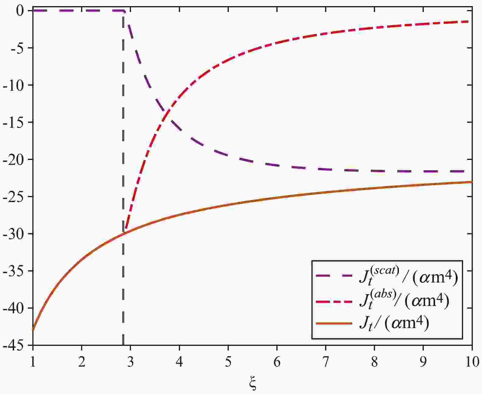
In Figs. 1 and 2, the components $ J_{\mu}^{({\rm{abs}})} $ and $ J_{\mu}^{({\rm{scat}})} $ and their sum $ J_{\mu} $ are numerically indicated by the parameters $ \beta = 1 $ and $ l = 0.05 $. Below the photon sphere, $ J_{\mu}^{({\rm{scat}})} $ vanishes for $ \xi< 3-3\,l $. Although the individual components $ J_{\mu}^{({\rm{abs}})} $ and $ J_{\mu}^{({\rm{scat}})} $ are not smooth, the total current $ J_{\mu} $ is smooth.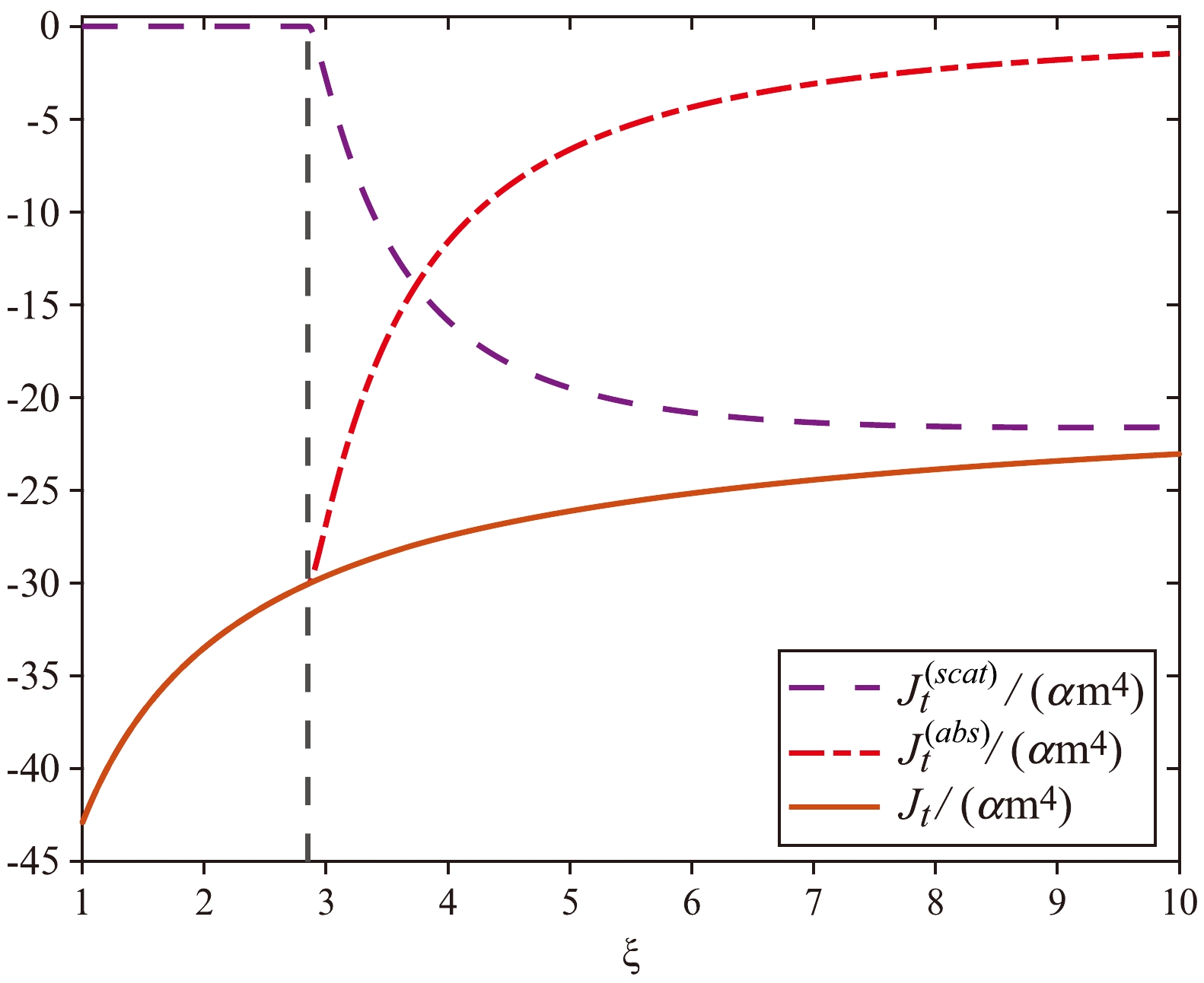

Figure 1.  (color online) Nonvanishing components $ J_{\rm{t}}^{({\rm{abs}})}/\alpha m^4 $, $ J_{\rm{t}}^{({\rm{scat}})}/\alpha m^4 $, and $ J_{\rm{t}}/\alpha m^4 $. The chosen parameters are $ \beta = 1 $ and $ l = 0.05 $. The vertical dashed black line represents the location of the photon sphere ($ \xi = 3(1-l) $).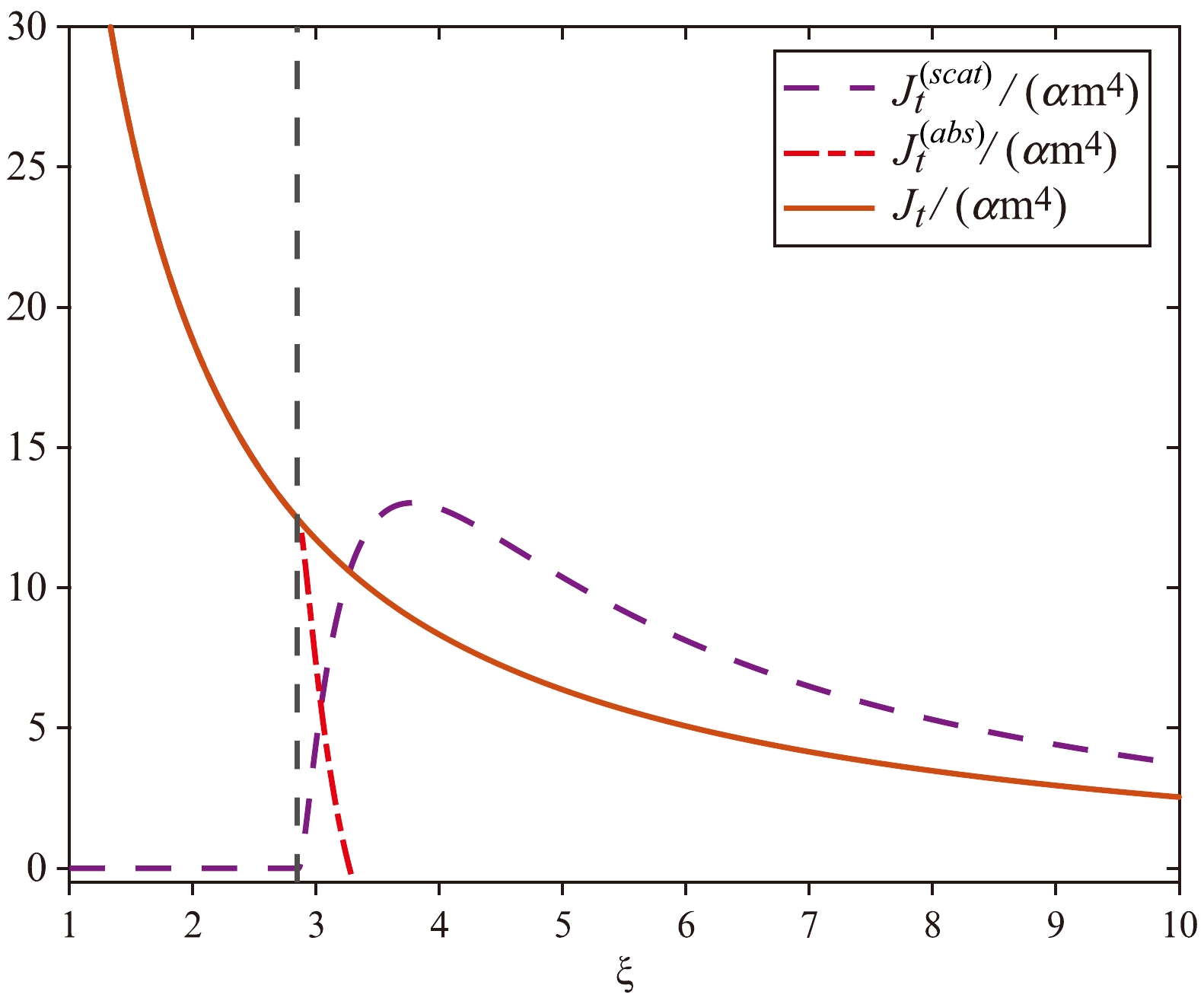

Figure 2.  (color online) Nonvanishing components $ J_{\rm{r}}^{({\rm{abs}})}/\alpha m^4 $, $ J_{\rm{r}}^{({\rm{scat}})}/\alpha m^4 $, and $ J_{\rm{r}}/\alpha m^4 $. The chosen parameters are $ \beta = 1 $ and $ l = 0.05 $. The vertical dashed black line denotes the location of the photon sphere ($ \xi = 3(1-l) $).

The particle number is defined as

A sample graph of $ n/n_{\infty} $ obtained for different values of l for $ \beta = 1 $ is plotted in Fig. 3. The figure shows that $ n/n_{\infty} $ decreases as the radius ξ increases. As illustrated, decreasing l increases the number of particles absorbed by the BH. The particle density of a BH with $ l>0 $ is lower than that of a Schwarzschild BH, while the particle density of a BH with $ l<0 $ is higher than that of a Schwarzschild BH.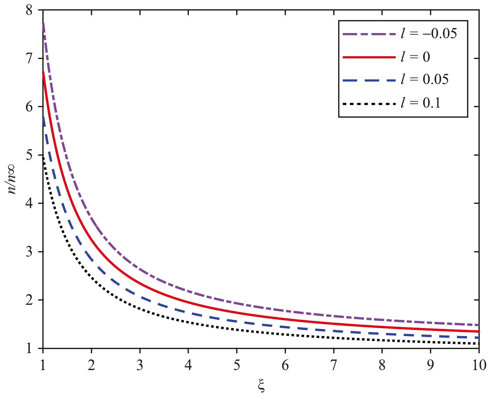

Figure 3.  (color online) The ratio $ n/n_{\infty} $ vs. ξ for $ \beta = 1 $ and $l = -0.05,\;0,\;0.05,\;0.1$

The conservation law of the particle density $ \nabla_{\mu}J^{\mu} = 0 $ can be written as

The particle accretion rate $ \dot{n} $ is defined by

where V represents the region of a BH, and S denotes the surface of the outer horizon. The vector $ \hat{n} $ = (1, 0, 0) is the unit vector normal to S directed outside.

The mass of the BH grows because of particles that are absorbed by the BH. Therefore, we define the mass accretion rate as

The mass accretion rate at the high temperature limit ($ \beta\to 0 $) is

Figure 4 displays a plot of $ \dot{M} $ against β for different values of l. The figure indicates that the accretion rate $ \dot{M} $ increases as l decreases. The accretion rate of Schwarzschild BHs is higher than those of BHs with parameters $ l > 0 $, and vice versa.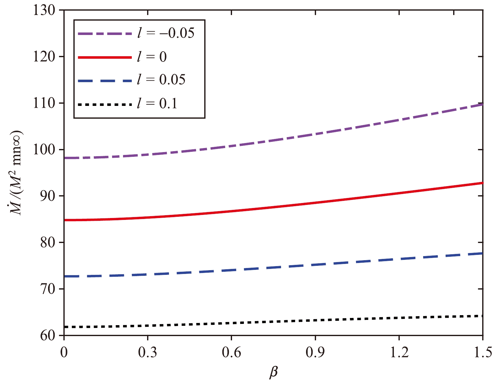

Figure 4.  (color online) Mass accretion rate $ \dot{M}/(M^{2}mn_{\infty}) $ vs. β for $ \beta = 1 $ and $l = -0.05,\;0,\;0.05,\;0.1$.

In [43], the metric of the Bumblebee BH is expressed as

where M is the mass of the black hole and l is also a constant characterizing the LSB. Figure 5 and Fig. 6 present comparisons of the mass accretion rates of the KR and Bumblebee BHs for fixed values of l. If $ l<0 $, the mass accretion rate of the KR BH is higher than those of the Schwarzchild and Bumblebee BHs. If $ l>0 $, the mass accretion rate of the KR BH is lower than those of the Bumblebee and Schwarzchild BHs. The mass accretion rate at the high temperature limit ($ \beta \to 0 $) for the Bumblebee BH is [43]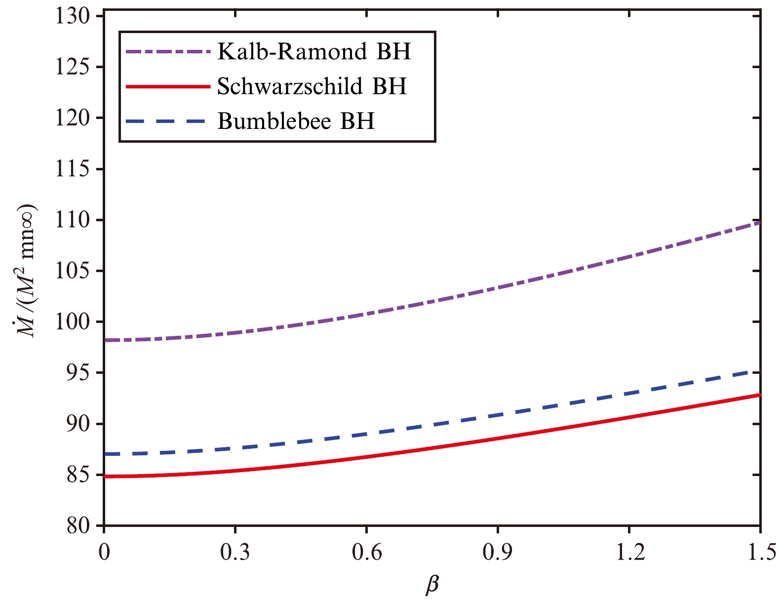

Figure 5.  (color online) Mass accretion rate $ \dot{M}/(M^{2}mn_{\infty}) $ vs. β for $ l = -0.05 $.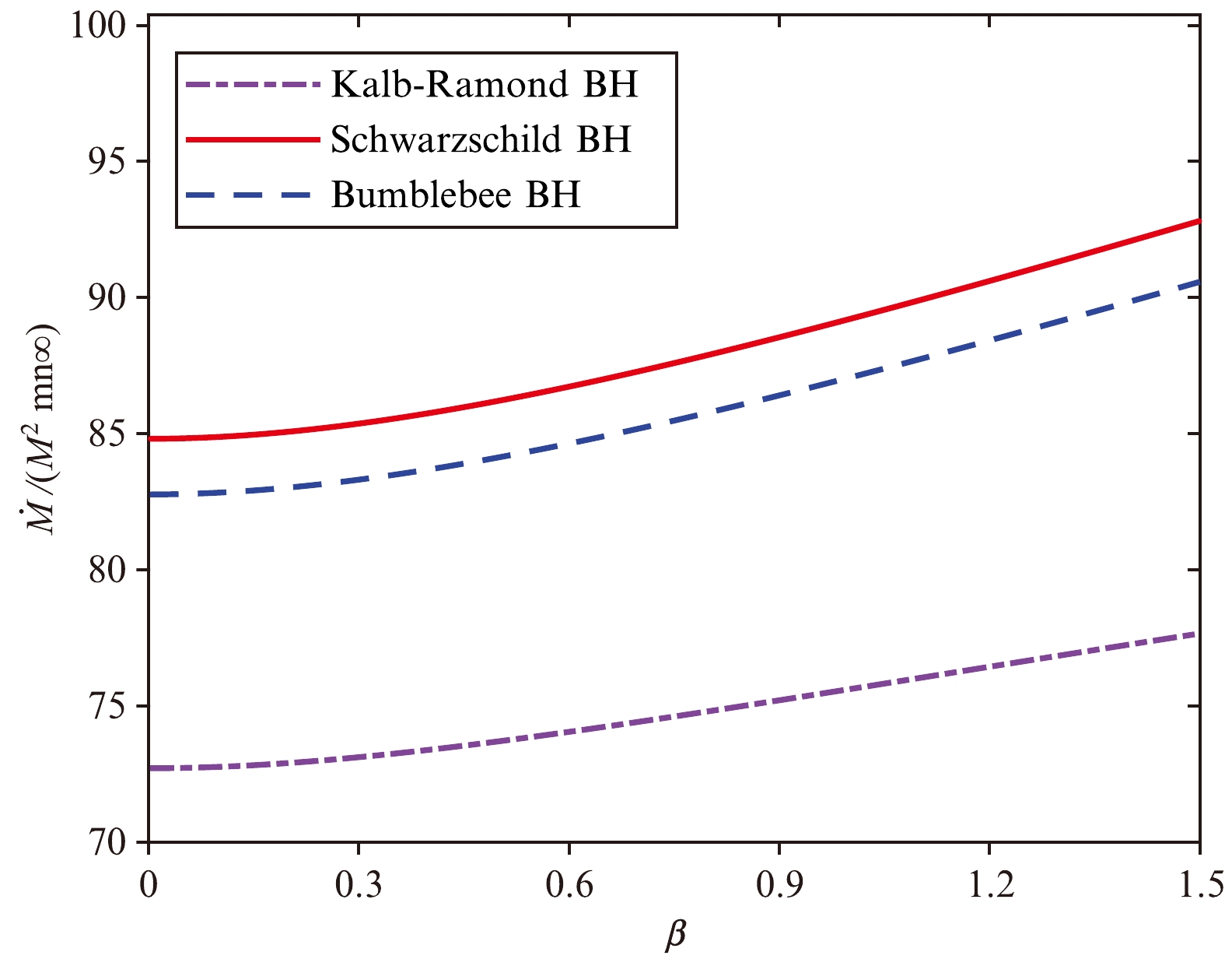

Figure 6.  (color online) Mass accretion rate $ \dot{M}/(M^{2}mn_{\infty}) $ vs. β for $ l = 0.05 $.

which is significantly different from Eq. (64). This can potentially be used to distinguish between KR and Bumblebee fields.

In this study, we introduced a model for the steady, spherically symmetric deposition of a Vlasov gas onto a BH within the gravitational backdrop of a KR field. Using the Maxwell-Jüttner distribution as the reference state at the boundary of the cosmos, we determined the particle current density $ J_\mu $ and the mass accretion rate $ \dot{M} $ for various values of the LSB parameter l. Our analysis of these accretion rate formulations showed a significant reliance on the model parameters: an increase in l was correlated with a decrease in the accretion rate. Additionally, we derived explicit formulations for the accretion rate within the high temperature limit ($ \beta \to 0 $). We also compared the accretion rate of a KR BH with that of a Bumblebee BH, and found that the results were different for the same value of l; this could be used to distinguish between KR and Bumblebee fields.

We considered the Maxwell–Jüttner distribution as an example of a gas distribution at infinity. In the future, we will explore observed quantities for different distribution functions , which may be more realistic. Furthermore, investigating the behavior of other BH archetypes using Hamiltonian formalism would be advantageous. Moreover, we can compute other quantities such as the energy-momentum tensor and energy accretion rate, comparing the results with those of perfect fluid models. Numerical methods such as Monte Carlo simulations could also be employed to investigate the accretion process of a Vlasov gas [53, 54].