Constraints on covariant Horava-Lifshitz gravity from precision measurement of planetary gravitomagnetic field

Quantum mechanics (QM) and Einstein's general relativity (GR) are two revolutionary developments in physics from the early 20th century. However, the incompatibility of these two theories has posed significant challenges for modern physics. Combining them to formulate a theory of quantum gravity remains elusive owing to numerous difficulties such as non-renormalizability and the nature of spacetime at small scales. Among the few candidate theories existing, Horava-Lifshitz gravity has attracted significant attention [1, 2].

Horava-Lifshitz gravity, proposed in 2009 [1], modifies the Einstein-Hilbert action by introducing higher-order spatial derivative terms. The primary motivation behind Horava-Lifshitz gravity is to construct a theory of quantum gravity that is renormalizable in the ultraviolet (UV) regime and resolves the limitations of standard GR. However, it is also anticipated that this theory may lose renormalizability and break down at extremely high energies, where quantum effects become dominant. To address these challenges, Horava and Melby-Thompson proposed a covariant version of Horava-Lifshitz gravity in 2010. By introducing an additional local U(1) symmetry, this modification resolved several undesirable features of the original theory, including infrared instability [1, 3] and strong coupling [4−7]. This covariant Horava-Lifshitz gravity is consistent with cosmology [8, 9]. Additionally, solar system tests have demonstrated consistency with observations when the gauge field and Newtonian pre-potential are incorporated into the metric [10].

Horava-Lifshitz gravity involves numerous parameters. However, when applied to the solar system, contributions from the cosmological constant and spatial curvature become negligible, leaving the solution dependent on only a few key parameters. Specifically, when the covariant form of Horava-Lifshitz gravity is expanded to the second post-Newtonian order, the potentials are determined by the gravitational constant G, the coefficient λ of the extrinsic curvature term characterizing deviations of the kinetic part of the action from GR, and two arbitrary coupling constants $ a_1 $ and $ a_2 $ in the matter action. To constrain these parameters, we conducted solar system experimental tests within the Parametrized Post-Newtonian (PPN) framework. PPN is a theoretical approach that approximates the effects of gravitational fields in various theories of gravity by incorporating parametrized post-Newtonian corrections [11]. With the help of the PPN formalism, all the parameters present in Horava-Lifshitz gravity are expressed in terms of PPN parameters [12]. Furthermore, these parameters can be constrained through the aforementioned solar system experiments.

A recent research focus has been leveraging gravitomagnetic effects to constrain the parameters of various gravity models. Within the weak-field approximation and slow-motion limit, the dynamics of the linearized Einstein field equations can be formally identified with that of Maxwell's equations [13−16]. Certain off-diagonal elements of the spacetime metric can be interpreted as the gauge potential in Maxwell's theory, thereby defining a gravitational analog of the magnetic field. Gravitomagnetism (GM) is a purely relativistic effect, and its measurement serves as an experimental test of gravity theories at a planetary scale. In this paper, we focus on the Lense-Thirring (frame-dragging) effect and aim to constrain the aforementioned Horava-Lifshitz parameters [17].

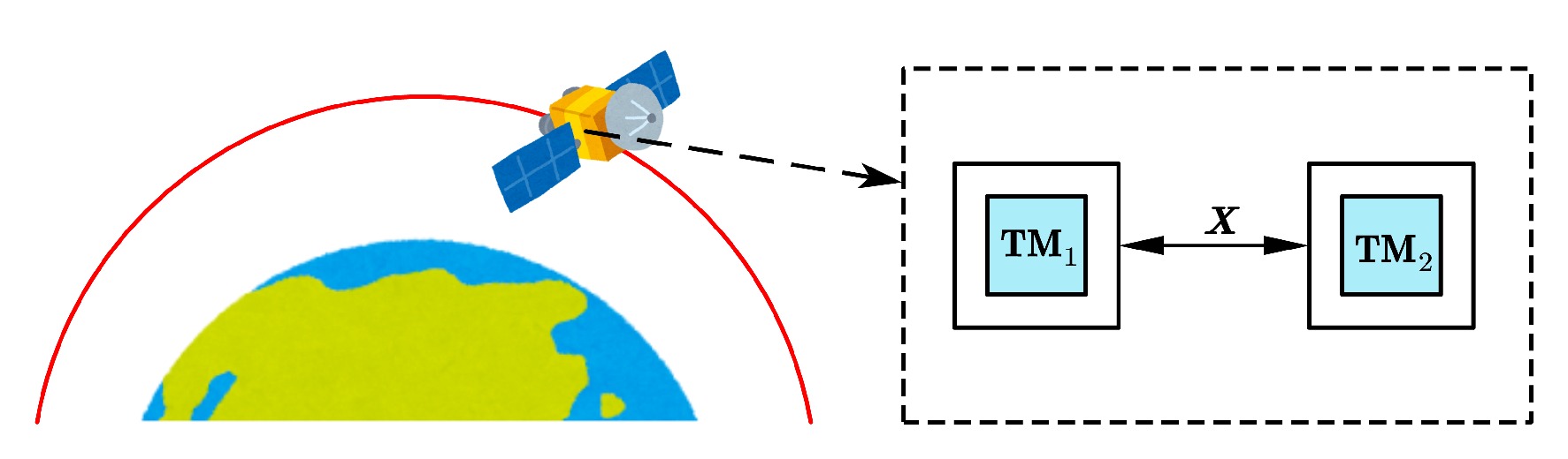
To date, experimental measurements of such physical effect have directly constrained the parameters of the Horava-Lifshitz theory [18]. The well-known Gravity Probe B (GP-B) experiment [19] measured the frame-dragging effect, constraining the difference between the gravitational constant G in Horava-Lifshitz theory and the Newtonian gravitational constant $ G_N $, yielding $ \left|\dfrac{G}{G_N}-1\right| \leq 0.05 $ and $ \left| \dfrac{2}{3}\left(\dfrac{G}{G_N}a_1-\dfrac{a_2}{a_1}-1\right) \right| \leq 0.0006 $. TheLaser Geodynamics Satellites (LAGEOS), launched by NASA (LAGEOS) and NASA-ASI (LAGEOS-2) [20], have also been employed to test the Lense-Thirring effect. Using laser-ranging techniques to measure distances, combined with the two LAGEOS nodal longitudes to eliminate uncertainties in the quadrupole moment of the Earth, this mission significantly improved sensitivity and constrained the parameter to a more precise value, $ \left|\dfrac{G}{G_N}-1\right| \leq 0.006 $. Furthermore, Monte Carlo simulations [21] constrained the combination of the Horava-Lifshitz gravitational constant G and Newtonian gravitational constant $ G_N $ to differ from unity by $ 2 \times 10^{-3} $. Unfortunately, for generic planetary sources, gravitomagnetic effects are several orders of magnitude weaker than Newtonian effects, posing a significant challenge for high-precision experimental measurements.

Considering the aforementioned difficulties and challenges, our current research aims to establish a new theoretical framework for the differential measurement of the planetary gravitomagnetic (GM) field using a space-based gradiometer. Unlike the standard readout of a gradiometer, which provides the differential acceleration between two test masses (TMs) [22, 23], this new design improves the detection precision. In theory, the GM field is part of the spacetime curvature and produces tidal forces acting on freely-falling TMs. Therefore the tidal force generated by the GM field can be directly measured through satellite gradiometry. As demonstrated in the LISA Pathfinder mission, the two free-falling TMs [24, 25] naturally constitute a one-dimensional gravity gradiometer. This raises the question of whether such a mission could also measure the GM field around a planet. Our studies demonstrate that by tracking the relative displacement of the two TMs in the direction transverse to the orbital plane (see Fig. 1), we can measure the GM field of the Earth through differential measurement and test classical solar system experiments. The basic schematic diagram is shown inFig. 1. During the on-orbit science phase, we track the relative motions of the two TMs, induced by the GM tidal force, using on-board laser interferometry. Specifically, at the second post-Newtonian level, the two TMs, located 50 cm apart and orbiting the Earth, follow trajectories governed by the Clohessy-Wiltshire equations derived from geodesic deviation. This occurs over a time scale shorter than the Lense-Thirring precession period ($ \sim 10^7 $ years) of the orbital plane. The tidal force generates a forced oscillation between the two TMs in the direction transverse to the orbital plane, enabling the differential measurement as well as the measurement of the GM field of the Earth. The paper is organized as follows. In Sec. II, we briefly review covariant Horava-Lifshitz gravity. In Sec. III, we solve the geodesic deviation equation up to the second post-Newtonian level for the two TMs located in the along-track direction of a nearly circular orbit. We identify the measurable signals generated by the GM field in Sec. III. In Sec. IV, we discuss the method for space-based gradient measurement and constrain the corresponding parameters of covariant Horava-Lifshitz gravity through this satellite experiment. Finally, discussion and conclusions are presented in Sec. V.

Figure 1.  (color online) A scheme to measure gravitational gradients using two TMs on satellites in orbit

In this paper, we study the Lense-Thirring effect in covariant Horava-Lifshitz gravity. It extends the symmetry of the Horava-Lifshitz gravity by introducing an additional U(1) gauge field as well as an scalar field. A generalized covariant theory of gravity is thus obtained which eliminates the extra degrees of freedom “spin-0 gravitons". Most importantly, it provides a general method for coupling gravity to other fields such as the matter field, which may cause Horava-Lifshitz gravity to differ from GR in the IR. Here, we focus on this new version, which includes the coupling λ in the extrinsic curvature term of the action [26, 27]. Explicitly, the gauge field $ A(t,x) $ and Newtonian pre-potential $ \phi(t,x) $ have been introduced to solve the scalar graviton problem. This theory satisfies the projectability condition, which means that the lapse function only depends on time, $ N = N(t) $. Considering all these aspects, the total gravitational action is given by [26, 27]

where $ g = \text{det}(g_{ij}) $ and

where $ {\cal{L}}_K $ is the kinetic energy term, and $ {\cal{L}}_\phi $ and $ {\cal{L}}_A $ are extra field terms. Here, the covariant derivatives as well as the Ricci terms are all refer to the three-metric $ g_{ij} $. The extrinsic curvature is represented by $ K_{ij} = g_i^k \nabla_k n_j $, where $ n_j $ is a unit vector normal to the spatial hypersurface; K is the trace of $ K_{ij} $. The three-dimensional generalized Einstein tensor is denoted by $ {\cal{G}}_{ij} = R_{ij} - \dfrac{1}{2} g_{ij} R + \Lambda_g g_{ij} $. We recognize R as the linearized Ricci scalar of $ g_{ij} $;$ \Lambda_g $ is the space curvature. The potential term $ {\cal{L}}_V $ refers to the potential part of the Lagrangian density [26, 27].

Matter coupling generalizes a scalar-tensor extension of the theory [10, 28], allowing the necessary coupling to emerge in the IR without compromising the power-counting renormalizability of the theory in the UV regime. Specifically, the matter action term is given by [26, 27]

where $ {\cal{L}}_M $ is the matter Lagrangian and $ \psi_n $ represents the matter fields. The metric and matter fields couple to the Arnowitt-Deser-Misner (ADM) components $\tilde{N},\;\tilde{N}_i,\;\tilde{g}_{ij}$ as defined in Refs. [26−28].

In the post-Newtonian approximations, we assume that the metric can be expressed in the form [12]

where $ \eta_{\mu\nu} ={\rm diag} (-1,1,1,1) $and

where $ {\cal{O}}(n) \equiv {\cal{O}}(v^n) $. It should be noted that, in contrast to GR, $ h_{ij} $ needs to be expanded to the fourth order in v to obtain consistent field equations for the Hamiltonian and momentum constraints, and for the trace part of the dynamical equations.

Based on the perturbation discussed in Eq. (4), given in Ref. [12], we have that

where the gauge freedom has been used to eliminate anisotropic terms in the space-space contribution of the perturbation. The coefficients are obtained at the appropriate order as follows:

where $ G_N $ is the Newton constant; $ G_N $ is in principle different from G; $ a_1 $ and $ a_2 $ are two arbitrary coupling constants in the matter action.

Before delving into the post-Newtonian calculations, let us first describe the physical framework underlying the proposed measurement scheme. We consider the simple case of a nearly circular orbit for a spacecraft (S/C) and and use the Earth-centered inertial frame as the reference frame for simplicity. The presence of the GM field induces the Lense-Thirring precession of the orbital plane around the rotation axis of the Earth (see Figs. 2 and 3). The precession rate of the orbital normal N relative to the Earth-centered inertial frame is given by [17]

Figure 2.  (color online) Illustration of frame-dragging effect.

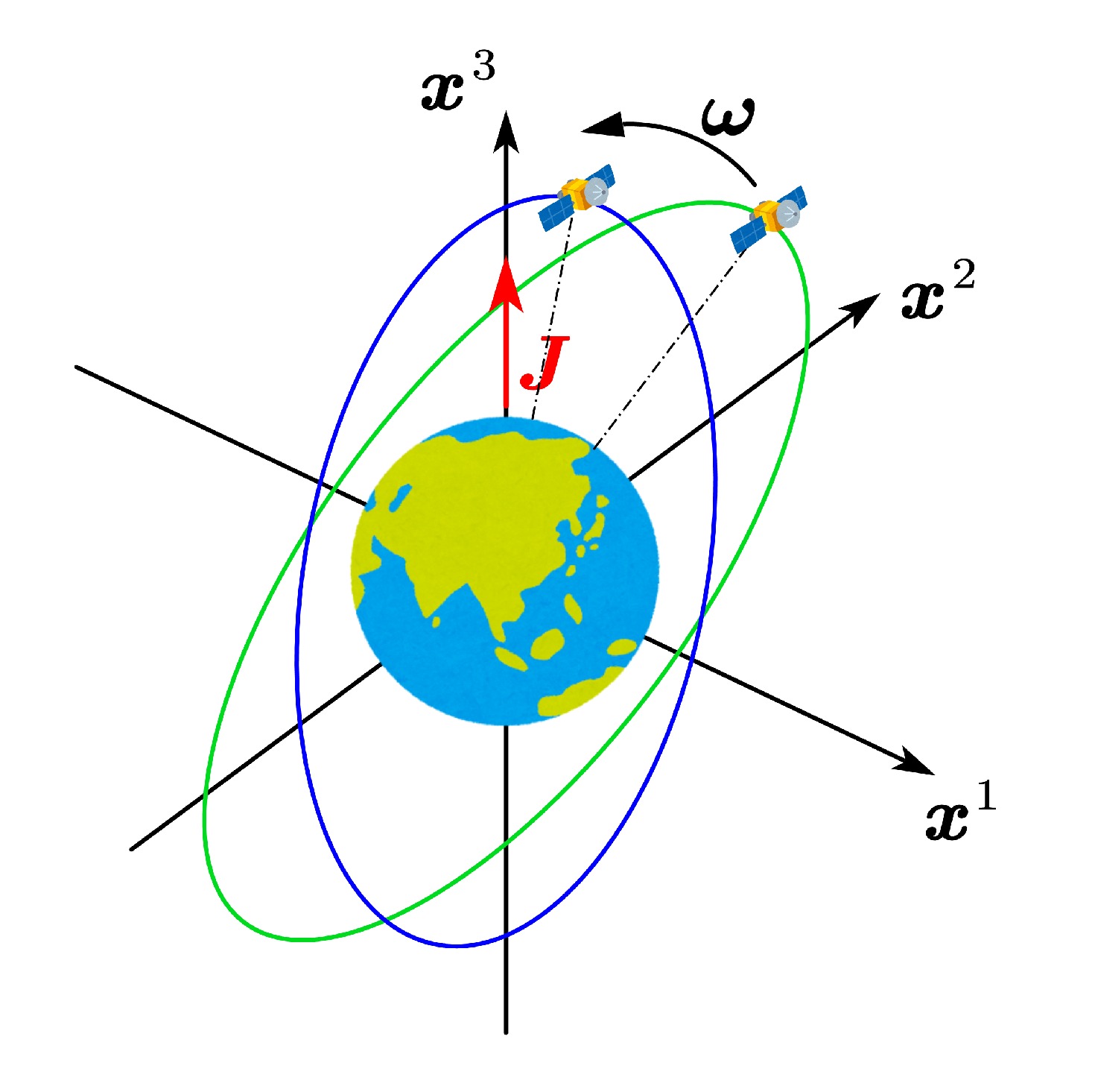
Figure 3.  (color online) Impact on the general satellite orbit by the frame-dragging effect.

where i is the orbital inclination. Simultaneously, the GM field also generates a precession of the orthonormal frame $ E_{(a)}^{i} $ attached to the S/C [29], which precesses around the rotation axis of the Earth with a different angular rate with respect to the Earth-centered inertial frame given by

Therefore, considering the two TMs as markers of the orbit, the projection of the position difference $ Z^i $ in the transverse direction enables measuring the difference in precession. This constant offset between these two precessing rates gives rise to a relative oscillation of the two TMs along the transverse direction of the S/C (see Fig. 4 and Fig. 5). Thus, the dominant GM signal in the S/C transverse direction $ E_{(3)}^{i} $ grows as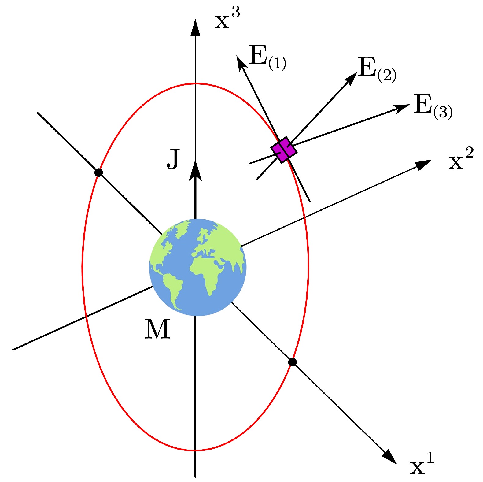

Figure 4.  (color online) LT precession of the polar, nearly circular orbit.

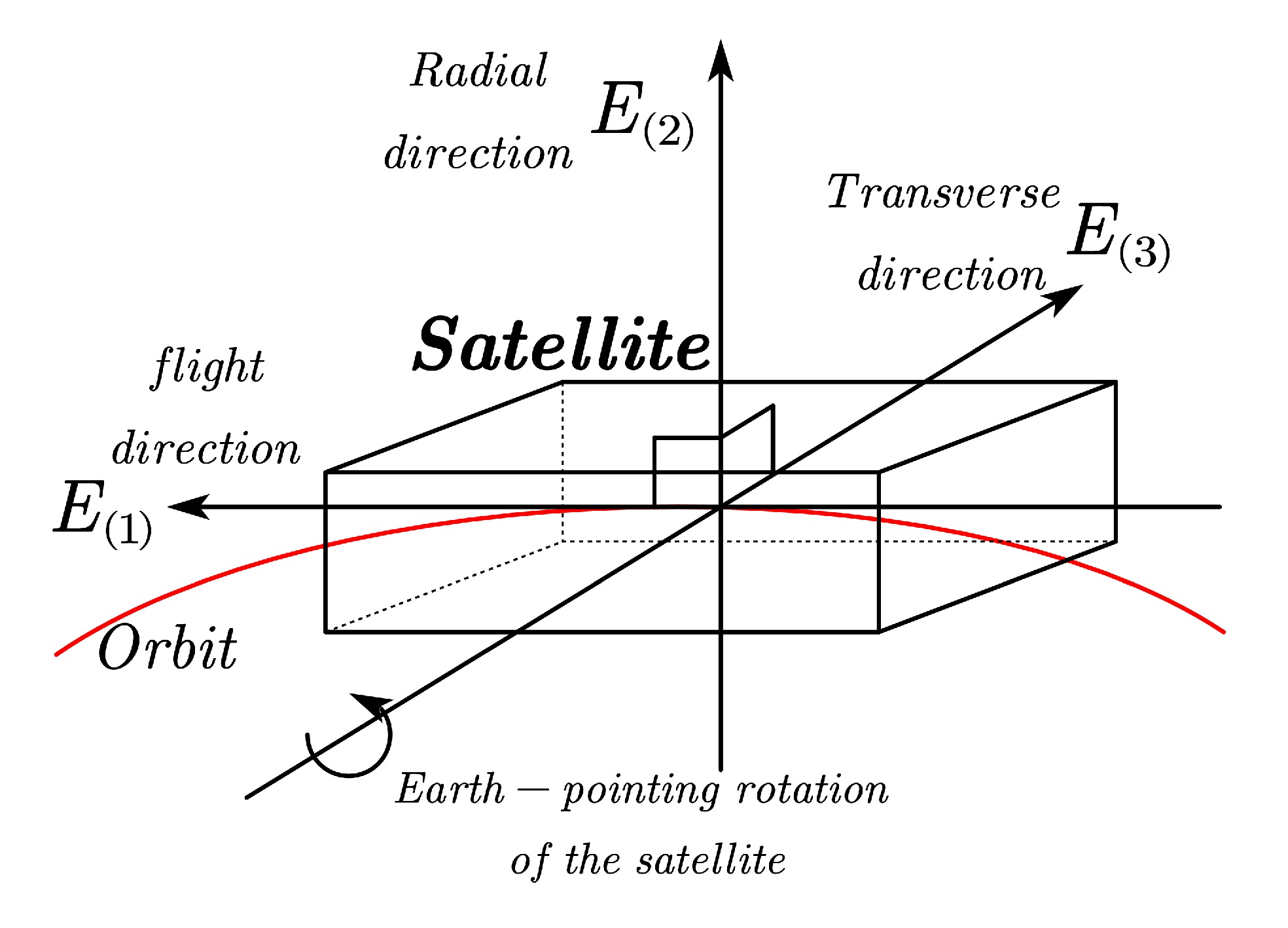
Figure 5.  (color online) Local frame: Earth pointing orientation of the satellite [30].

where ω is the orbital frequency. Owing to this differential GM signal, the uncertainty (measurement error) in determining the globally fixed reference system is not relevant to the proposed experiment.

By measuring the relative displacement of the TMs in the transverse direction using on-board laser interferometry, the frame-dragging precession can be tracked with high precision. This approach differs from the LAGEOS or LARES missions, which track the orbital plane precession of a satellite by observing variations in the Keplerian elements with respect to the geocentric frame. Moreover, given that the GM precession is referenced to a globally defined inertial frame, it measures the differential precession of two gyroscopes: the rolling S/C along the orbit and the orbit of the S/C itself. This differential measurement circumvents many technical challenges associated with defining a global reference frame, such as those encountered in the GP-B experiment. Next, we will present the detailed derivations of the second-order post-Newtonian geodesic equations for the relative motion between the free-falling TMs in the local frame of the S/C.

Based on the above discussion, the two freely-falling TMs in the along-track direction naturally form a one-dimensional gravity gradiometer. This setup enables measuring the relative acceleration of the two TMs induced by the tidal gravitational force acting between them. To proceed with our calculations, we need to specify the orbit and the local tetrad shown in Figs. 4 and 5. Here, we consider a polar orbit as an example. Specifically, the 1PN (first-order post-Newtonian) approximation for a nearly circular (spherical) orbit can be derived as follows:

The initial longitude of the ascending node is zero, and the true anomaly is given by $ \Psi = \omega \tau $, where a denotes the orbit radius and ω represents the mean angular frequency relative to the proper time along the orbit. The 1PN local tetrad $ E_{(a)}\ ^{i} $ up to the first-order post-Newtonian shown in Figs. 4 and 5 can be derived as follows [30]:

where $ \eta = \dfrac{G}{G_N} = -\dfrac{k}{4} $. With the local tetrad $ E_{(a)}^{i} $ obtained, the geodesic deviation can be explicitly expanded as

where $ X^i = X^{(a)} E_{(a)}^i $ and $ \gamma^{(a)}_{\ (b)(c)} = E^{(a)}(\bigtriangledown_i E_{(b)j})E^i_{(c)} $ are the Ricci rotation coefficients. The first two terms in Eq. (12) represent the Coriolis and inertial tidal forces, which originate from the relative rotation of the local frame of the spacecraft with respect to the parallel propagated frames. The last term accounts for the tidal force generated by the spacetime curvature.

With all the results in place, we substitute the relevant quantities into the geodesic deviation expressed by Eq. (12). By retaining the 1PN terms and neglecting contributions beyond $ \dfrac{X^{(a)}}{a^2} {\cal{O}}(\epsilon^4) $ and $ \dfrac{X^{(a)} \Psi}{a^2} {\cal{O}}(\epsilon^4) $ $ (\epsilon = \dfrac{M}{r} $ is approximately $ 10^{-5}\sim 10^{-6} $), and after some algebraic manipulations, the time component of the geodesic deviation equation in the local frame of the spacecraft is trivial, as expected:

and the spital parts may be expressed in an elegant form as follows:

These equations are the basis for our next measurement. In the proposed measurement scheme, two TMs are positioned in the along-track direction with a separation distance of $ d \sim 50 $ cm and follow a nearly circular orbit of radius a. Therefore, we can assume initial conditions with slight misalignments and deviations from the along-track orientation as

Under these conditions, Eqs. (14)−(16) are further simplified as

These equations agree well with the physical framework of a transverse forced harmonic oscillator. Solving the above differential equations, we obtained the targeted signals as follows:

Eqs. (22)−(24) represent the signal that we aim to measure using a high-precision gravity gradient measurement mission. The oscillation amplitude, which grows linearly over time, can be measured by superconducting gradiometers. From the perspective of frame-dragging precessions, this growing oscillation is generated by the differential precession of the orientation of the spacecraft and the orbital plane around the rotation axis of the Earth. This contrasts with the GP-B mission and the LAGEOS/LARES experiments, which attempted to measure frame-dragging effects with respect to a globally defined reference frame. Furthermore, this differential precession method enhances measurement accuracy, which will be discussed in detail in the next section.

Currently, two highly promising schemes exist for enhancing the accuracy of gravity gradient measurements: the superconducting and laser gravity gradiometers. Both technologies represent cutting-edge advancements with distinct advantages in improving the accuracy and precision of gravity gradient measurements. Each approach leverages advanced principles of physics and engineering to overcome traditional measurement limitations, making them invaluable tools in modern scientific research and applications.

The superconducting gravity gradiometer utilizes advanced superconducting technology to measure gravity gradients. At its core is a superconducting accelerometer, which operates based on the magnetic interaction between a current-carrying coil and a superconductor in a fully diamagnetic Meissner state. This configuration creates a magnetic spring oscillator that harnesses the Meissner effect, zero-resistance effect, and Josephson macroscopic quantum effect of superconductors, enabling highly sensitive micro-displacement detection. One of the key advantages of the superconducting gravity gradiometer is its exceptionally low internal noise, which surpasses the measurement resolution limits of traditional room-temperature instruments.

The laser gravity gradiometer relies on the principle of dual-path interference. It measures the rate of change of gravity across a three-dimensional space by employing two laser interferometric absolute gravimeters arranged differentially. This configuration allows the instrument to measure the gravitational acceleration of two falling bodies relative to their respective reference points using laser interferometry. By analyzing the positional shifts of these bodies, the instrument calculates the gravity gradient at the measurement points through differential computations. The differential measurement performed by a laser gravity gradiometer helps reduce errors caused by vibrations, significantly enhancing measurement precision. Additionally, with slight adjustments to the optical path and positions of the falling bodies, the system can be adapted to measure transverse gravity gradients.

In the baseline design of highly sensitive gravity gradiometers operating in microgravity or zero-g environments in space, electrostatic or superconducting devices are commonly used. In these systems, pairs of proof masses are typically aligned along each measurement axis, with a separation of approximately 50 cm. To mitigate disturbances that may affect the proof masses, various strategies for isolation, position sensing, and control combinations are implemented, as extensively reviewed in [22, 23, 31]. A superconducting gravity gradiometer (SGG) consists of two (or more) superconducting accelerometers, each comprising a superconducting TM, a superconducting sensing coil carrying a persistent sensing current, and a SQUID. Gravity (or other forces) causes the TM to move, modulating the inductance of the mass-coil system due to the Meissner effect. According to flux quantization, the sensing current adjusts to maintain a conservative flux, generating a current signal that is detected by the SQUID. [32]. To measure gravity gradients and reduce common-mode noise such as satellite drag and temperature fluctuations, the two TMs are coupled with a superconducting sensing circuit shown in Fig. 6.

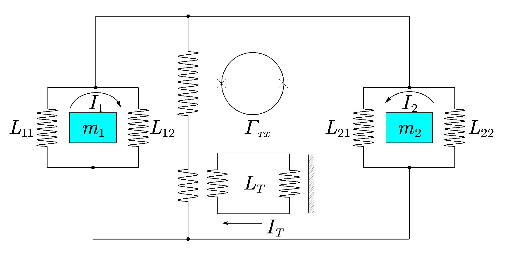
Figure 6.  (color online) Principle of superconducting differential acceleration sensing [32].

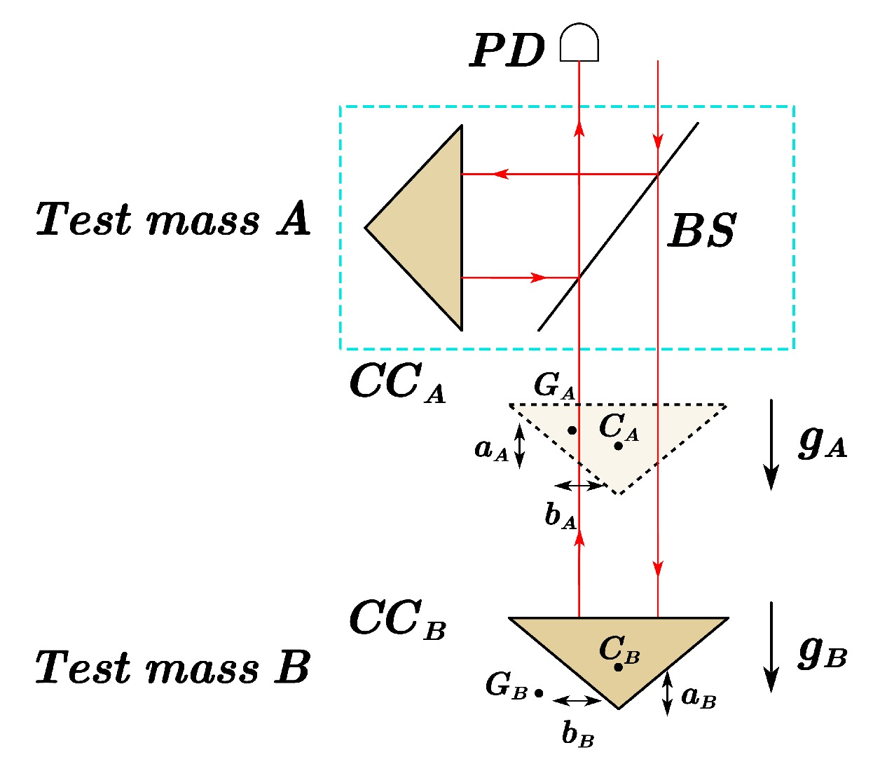
Figure 7 depicts the schematic optical layout of the laser interferometers [33]. Two TMs, namely A and B, are simultaneously dropped from different heights within a vacuum chamber and experience gravitational fields $ g_A $ and $ g_B $, respectively. A laser beam aligned vertically is directed onto a cube beam splitter (BS) embedded in TM A. The BS splits the laser beam into two arms: one reflects off a corner-cube prism $ CC_A $ embedded in TM A, and the other reflects off a corner-cube prism $ CC_B $ embedded in TM B. These reflected beams are recombined at the BS, forming interference fringes based on relative optical-path changes. The interference fringes are detected by a photodetector (PD) located outside the vacuum chamber. The difference in free-fall acceleration ($ \Delta g = g_B - g_A $) between the two TMs is determined by analyzing these interference fringes [33]. Solid glass corner-cube prisms are preferred for Laser Interferometric Gravity Gradiometers (LIGGs) owing to their availability and ease of integration within the TMs. [33].

Figure 7.  (color online) Principle of laser interferometer [33, 34].

In this paper, we consider a single-satellite mission in Earth orbit. The satellite platform is ultra-stable and ultra-quiet, with drag-free control. Its payload includes a dual-axis high-precision laser interferometer for measuring gravitational gradients and a high-precision star-to-ground time-frequency comparison system. The satellite orbits in a 1500-km-altitude Sun-synchronous circular orbit, maintaining a nadir-pointing attitude towards Earth. By utilizing data from the gradient meter, the satellite achieves two-degree-of-freedom drag-free control along the flight and orbit normal directions, ensuring optimal operation of the gravitational gradient instrument.

Here, we explain how to constrain our parameters in detail. For an orbital altitude of 1500 km, the orbital angular frequency is $ \omega = 9 \times 10^{-4} $ rad/s. We consider gradiometers with a sensitivity of approximately 0.1 mE, which corresponds to an orbital frequency $ f = \sqrt{GM/a^3} = 0.144 $ mHz. Over one year's accumulation, the number of total cycles in the signal data amounts to $ 4.5 \times 10^3 $. Therefore, for gradiometers with sensitivity better than $ 10^{-2} $ mE/$ \sqrt{\text{Hz}} $ in the low-frequency band near $ 0.1 $ mHz [35], we could implement a proper and narrow bandpass filter, optimized for the signal frequency, to effectively eliminate unwanted noise and errors. Given that the signal is periodic, a one-year dataset could then potentially reveal a noise floor of approximately $ 10^{-5} $ mE. If we set a suitable signal-to-noise ratio threshold for a one-year measurement period of the secular signal, considering the displacement between TMs due to noise during the test, we expect the following constraint on the parameter η: $ \left | \eta - 1 \right | = \left | \dfrac{G}{G_N}-1 \right | = 0.0025 $. For optical gradiometers based on the new generation of space gravity gradiometer missions, constraints on such parameters may yield similar or even stronger bounds.

In this paper, we have explored the weak-field and slow-motion limit of a covariant version of Horava-Lifshitz theory to constrain its parameters based on recent space experiment results. This approximation is particularly effective in describing gravitational fields around Earth. It is anticipated that future gravity gradient measurement missions will provide more accurate data, enabling more precise constraints and a deeper scrutiny of modified gravity theories, such as Horava-Lifshitz Gravity, which extend beyond Einstein's GR.

Our analysis demonstrates that high-precision laser gradiometers have the potential to improve the precision of parameter constraints by one or two orders of magnitude. Specifically, for a gravitational gradient detection mission with an orbital altitude of 1500 km and an expected mission duration of one year, the use of a new generation of equipment with higher accuracy than existing technologies could significantly enhance the precision of the measurements to $ 10^{-2} $ mE/$ \sqrt{\text{Hz}} $ at the predetermined detection frequency, thereby establishing stronger constraints on the modification of the gravitational theory. Considering the Horava-Lifshitz theory described in this paper as an example, the constraint $ \left|1-\dfrac{G}{G_N}\right| $ can reach $ 0.0025 $.This represents a significant advancement over previous methods, such as the Gravity Probe B (GP-B) experiment and the LAGEOS satellites, which have already provided valuable constraints on the parameters of the Horava-Lifshitz theory. The innovative method here proposed, using laser interferometry in space, offers a new approach for precisely constraining parameters such as G, the gravitational constant, within the framework of the Horava-Lifshitz theory.

The proposed method for measuring the GM field through differential measurement of the relative motion of two TMs in space is a promising approach. It enables the direct measurement of the tidal force generated by the GM field, which is a component of the spacetime curvature. This method differs from previous efforts that attempted to track the orbital plane precession of a satellite by observing variations in the Keplerian elements with respect to the geocentric frame.

Furthermore, this study establishes a new theoretical framework for the differential measurement of the planetary GM field using a space-borne gradiometer. This framework is essential for the design and implementation of future space missions conceived for measuring gravitational gradients with unprecedented precision. The potential of such missions is vast, offering significant opportunities to test and constrain theories of gravity, including Horava-Lifshitz gravity.

In conclusion, the combination of advanced measurement techniques and theoretical frameworks presented in this paper opens new possibilities for the study of gravitational phenomena on a planetary scale. The pursuit of these research lines will not only refine our understanding of gravity but also contribute to the broader quest for a unified theory of quantum gravity.