Critical collapse of massless scalar fields in asymptotically anti-de Sitter spacetime

Critical collapse plays a crucial role in theoretical and numerical research, offering insights into the nature of spacetime singularities. It is classified into two types based on black hole mass behavior: Type I, characterized by a finite minimum mass, and Type II, allowing for arbitrarily small masses. Choptuik's seminal work [1] first revealed the Type II critical phenomena through numerical simulations of spherically symmetric massless scalar fields. He identified critical value $p^{*}$ in the initial data parameter, p. For $p>p^{*}$, collapse results in black hole formation, whereas for $p<p^{*}$, the field disperses to infinity. At slightly greater than $p^{*}$, the black hole mass follows the power law: $M_{\rm BH} \propto (p-p^{*})^{\gamma}$, where $M_{\rm BH}$ is the mass of the black hole and $\gamma \approx 0.37$ is a universal constant independent of the initial data. Additionally, the critical solution exhibits an echoing period with $\Delta \approx 3.44$. Type I collapse was later discovered by Choptuik et al. in Yang-Mills field numerical simulations [2]. Subsequent research has broadened the scope of gravitational collapse studies, including various matter [3–20], higher dimensions [21–25], modified gravity theory [26–30], and axisymmetric configurations [31–34]. For a comprehensive review on gravitational collapse, refer to Refs. [35, 36].

Pretorius et al. examined the gravitational collapse of an axially-symmetric massless scalar field in $(2+1)$-dimensional anti-de Sitter (AdS) spacetime [37]. Their research revealed that the exterior geometry approached the BTZ solution, whereas a strong, spacelike curvature singularity formed within the event horizon. They also observed a continuous self-similar solution and black hole mass exponent of approximately 1.2. Husain et al. investigated the critical collapse of a spherically symmetric massless scalar field under various negative cosmological constants [38], concluding that the critical exponent is independent of the cosmological constant.

Bizoń and Rostworowski investigated the nonlinear evolution of a spherically symmetric massless scalar field in AdS spacetime [39]. Their research revealed that even small perturbations will eventually form a black hole after multiple reflections at the outer boundary. Oliv'an et al. numerically explored the critical collapse of the massless scalar field in AdS spacetime [40], uncovering a series of critical points with discretely self-similar dynamics and a power law of the mass gap. Subsequent research has further probed the AdS instability conjecture [41–50]. In this study, we focus exclusively on the critical phenomena of the initial collapse under varying cosmological constants, disregarding the influence of outer boundary reflections.

Vera explored the critical collapse of massless scalar fields in asymptotically AdS spacetime [51], disregarding outer boundary reflections. His study of critical phenomena under varying cosmological constants revealed a relationship between critical amplitude $A^{*}$ of the initial scalar field and AdS radius L:

where $A^{*}_{\infty}$ denotes the critical amplitude of the initial scalar field in asymptotically flat spacetime. Undetermined function f depends on L and potentially on scalar field's center $v_{0}$ and width σ. Our findings suggest a linear relationship between $A^{*}$ and cosmological constant Λ, and the slope of this relationship is influenced by the initial conditions.

This paper is structured as follows. In Sec. II, we outline the methodology used to simulate the collapse of massless scalar fields in asymptotically AdS spacetime. In Secs. III and IV, we discuss the critical collapse and behavior of the critical amplitude as changes in width and position, respectively. The results are summarized in Sec. V. Throughout this paper, we set $c=1$ and $G=1$.

We consider the collapse of massless scalar field ϕ in asymptotically AdS spacetime. The action is

where R is the Ricci scalar and Λ represents the cosmological constant. Applying the variational principle to the action with respect to both the metric and scalar field yields the following equations:

Energy-momentum tensor $T_{\mu\nu}$ for the scalar field is

We use the double-null coordinates,

where r is the area coordinate. For simplicity, we introduce $\Lambda=-3/L^{2}$, with L denoting the AdS radius. Combining Eqs. (2) and (5) yields the following field equations:

where $(_{,u})$ and $(_{,v})$ represent the partial derivatives with respect to u and v, respectively. The equation of motion for the scalar field, derived from Eq. (3), is

For convenience, we introduce new variables s, p, q, c, d, f, and g defined as

These variables allow us to reformulate the system as a set of first-order coupled partial differential equations. Consequently, Eqs. (6)−(10) can be rewritten as

The initial values for d and q are given by

where A, σ, and $v_{0}$ denote the amplitude, width, and central position of the initial scalar field, respectively. Boundary conditions are imposed along the $u=v$ axis, where we set $r=0$ and $f=-g$. From Eqs. (17) and (18), we derive $a=2g$ and $p=q$. Owing to the requirement for continuity at the center, we also impose $a_{,r}=0$ and $s_{,r}=0$. We set the initial conditions for d and the terms related to L in the equations of motion to zero in asymptotically flat spacetime.

The Hawking mass is defined as

Additionally, we introduce proper time T on the $u=v$ axis as

Our numerical approach integrates Eqs. (11), (13), (14), and (18) using a fourth-order Runge-Kutta method, whereas Eqs. (17) and (19) are evolved through a predictor-corrector algorithm. For comprehensive simulation details, refer to Refs. [6, 51, 52].

The spatial domain in all simulations is discretized using $10^{4}$ grid points with a $10^{-3}$ interval. Black hole formation is signaled by $g<10^{-4}$, triggering code termination. We employ the bisection method to pinpoint the $A^{*}$ value to 12 significant figures, fixing other parameters throughout this process.

We describe the collapse of a spherically symmetric massless scalar field by evolving Eqs. (12)−(19). Fixing $v_{0}$, we employ the bisection method to determine critical amplitude $A^{*}$ for different σ and L.

Figure 1(a) shows the variation in scalar field s along the $u=v$ axis with respect to $\ln(T^{*}-T)$, where $T^{*}$ denotes the time of naked singularity formation. We observe similar echoing periods across different σ by combining Table 1. Figure 1 (b) demonstrates the power-law behavior of black hole mass for various σ in the supercritical regime, revealing nearly identical critical exponents. Consistently, we find an echoing period of $\Delta \approx 3.4$ and a critical exponent of $\gamma \approx 0.37$, independent of σ and L.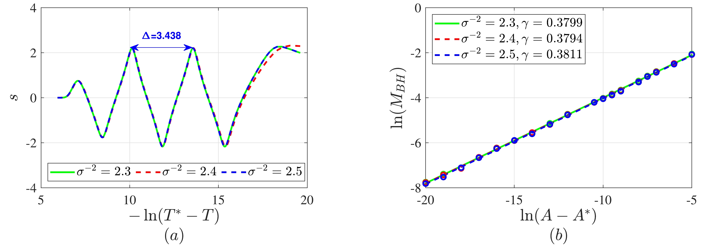

Figure 1.  (color online) Critical phenomena of massless scalar field collapse in asymptotically flat spacetime. (a) Evolution of scalar field s along the $u=v$ ($r=0$) axis. (b) Power-law of black hole mass. Initial parameter in Eq. (21): $v_{0}=2$. See Table 1 for specific details.

$\sigma^{-2}$	$A^{*}$	Δ	γ
$2.3$	$0.0495129325914$	$3.436$	$0.3799$
$2.4$	$0.0489338996341$	$3.441$	$0.3794$
$2.5$	$0.0483713656140$	$3.438$	$0.3811$

Table 1.  Critical amplitude $A^{*}$(second column), echoing period Δ (third column), and critical exponent γ (fourth column) of the initial scalar fields with different widths in asymptotically flat spacetime. The initial condition in Eq. (21) is $v_{0}=2$. (Critical amplitude is retained with twelve significant figures, and the echoing period and critical exponent with four significant figures).

Vera's study of the critical collapse in AdS spacetime revealed a relationship between critical amplitude $A^{*}$ and AdS radius L (as shown in Fig. 2):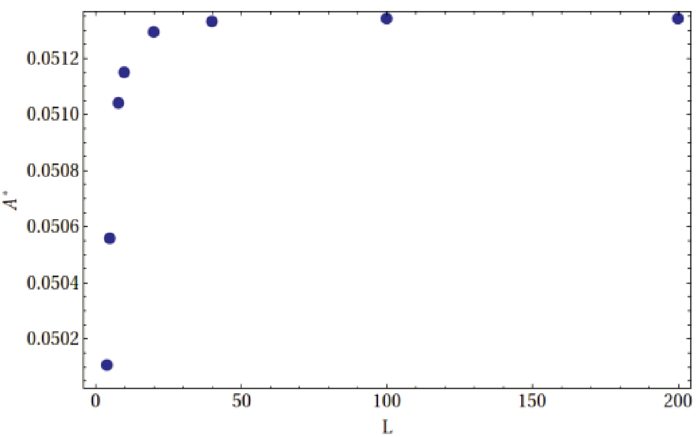

Figure 2.  (color online) Critical amplitude $A^{*}$ in the initial scalar profile Eq. (21) vs. AdS radius L. (Figure 5.17 in Ref. [51]).

where $A^{*}_{\infty}$ represents the critical amplitude in asymptotically flat spacetime. Undetermined function f is a function of L and possibly a function of $v_{0}$ and σ.

Our analysis, presented in Fig. 3 (a), reveals a linear relationship between critical amplitude $A^{*}$ and cosmological constant Λ for a fixed σ: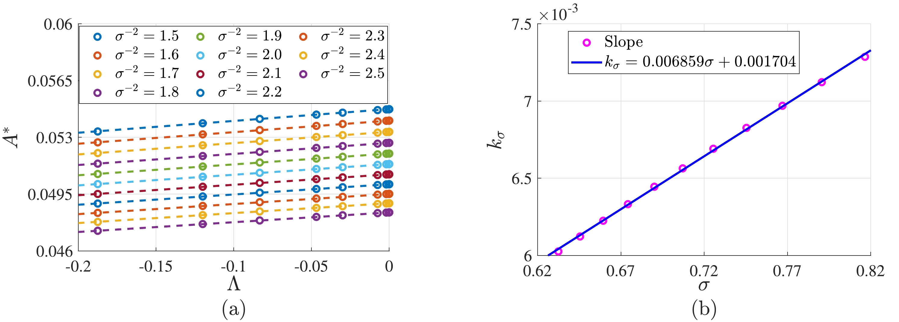

Figure 3.  (color online) Relationships among critical amplitude $A^{*}$ of the initial scalar field, cosmological constant Λ, and width of the initial scalar field σ. (a) $A^{*}$ vs. Λ. The initial condition in Eq. (21) is $v_{0}=2$. (b) $k_{\sigma}$ vs. σ.

Furthermore, Fig. 3 (b) shows that slope $k_{\sigma}$ exhibits a linear relationship with σ,

Combining Eqs. (25) and (26), we derive

Employing the aforementioned method, we study the critical collapse under varying $v_{0}$ and L. Consistently, we observe an echoing period of $\Delta \approx 3.4$ and a critical exponent of $\gamma \approx 0.37$ across different $v_0$ and L. These results are in agreement with Choptuik's findings in [1].

Figure 4 (a) reveals a linear relationship between $A^{*}$ and Λ for a fixed $v_{0}$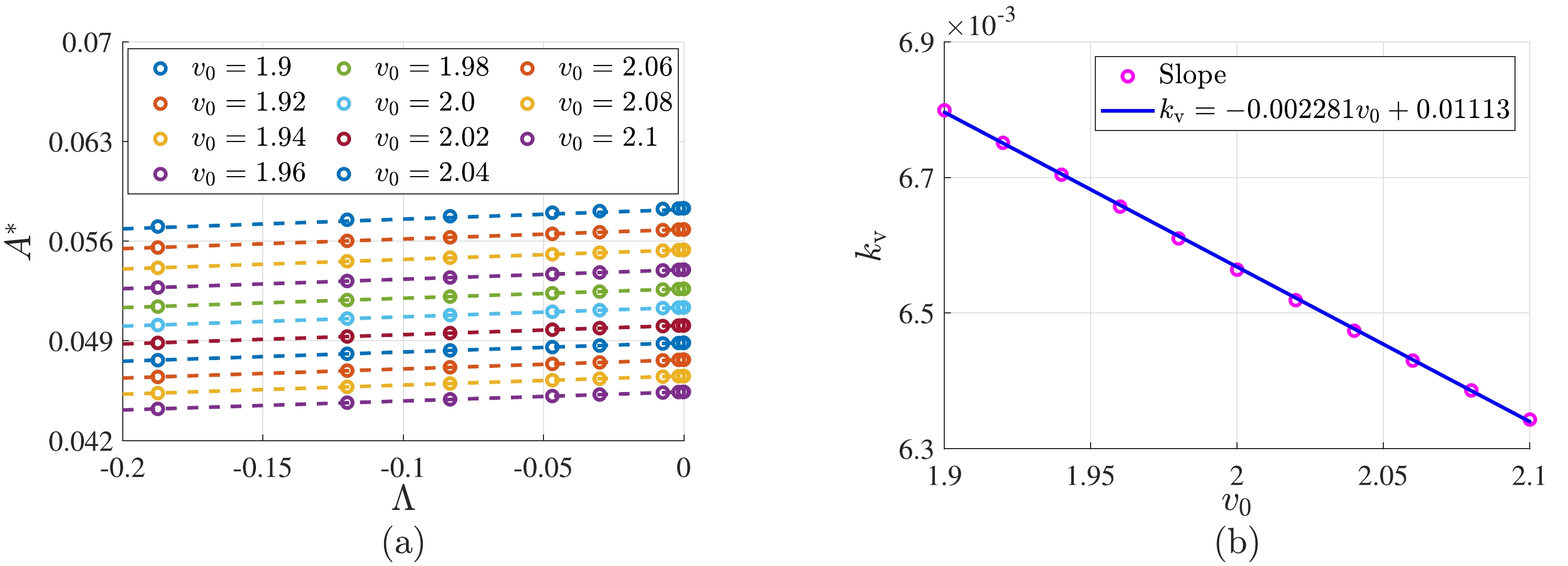

Figure 4.  (color online) Relationships among critical amplitude $A^{*}$ of the initial scalar field, cosmological constant Λ, and position of the initial scalar field $v_{0}$. (a) $A^{*}$ vs. Λ. The initial condition in Eq. (21) is $\sigma^{-2}=2$. (b) $k_{\text{v}}$ vs. $v_{0}$.

Furthermore, Fig. 4 (b) demonstrates a linear relationship between slope $k_{\text{v}}$ and $v_{0}$

Combining Eqs. (28) and (29) yields

Figures 3 (b) and 4 (b) show that slope $k_{\sigma}$ increases with σ, whereas slope $k_{\text{v}}$ decreases with $v_{0}$. Integrating these datasets produces Fig. 5, leading to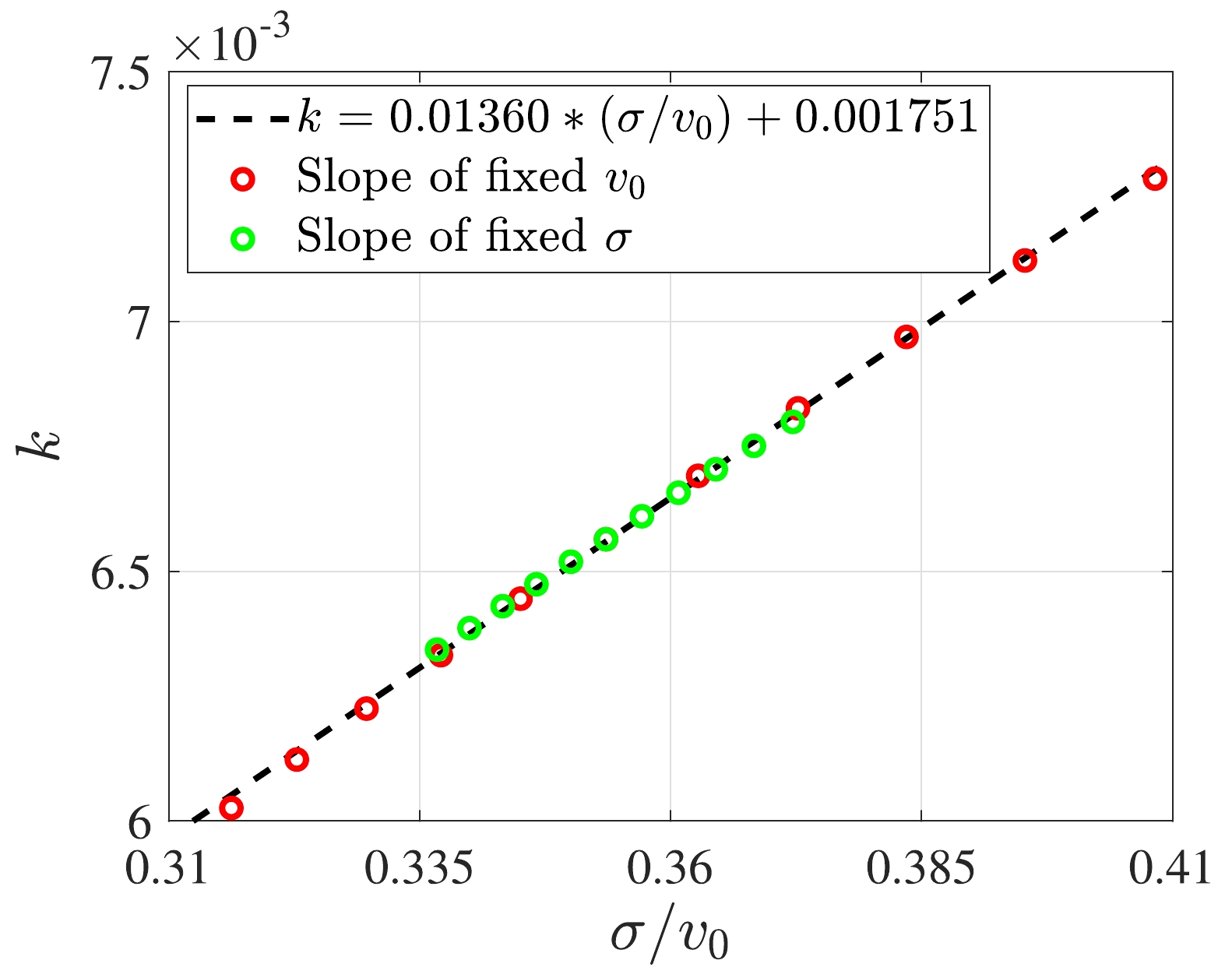

Figure 5.  (color online) Linear relationship between slope k and initial condition $\sigma/v_{0}$.

We performed numerical simulations of critical collapse involving spherically symmetric massless scalar fields under various initial scalar field profiles. Our results showed echoing periods and critical exponents consistent with Choptuik's findings across different initial conditions and cosmological constants. Furthermore, we found that Vera's fitting result in Eq. (24) relating critical amplitude $A^{*}$ to AdS radius L can be replaced by a linear relationship, Eq. (31), between critical amplitude $A^{*}$ and cosmological constant Λ ($\Lambda=-3/L^{2}$). Additionally, by manipulating the width and position of the initial scalar field, we demonstrated that the slope characterizing this linear relationship exhibits linear dependence on the initial conditions. Finally, we proposed a concise formula to describe the relationship between the critical amplitude of massless scalar fields in asymptotically AdS spacetime and the initial configuration of the scalar field. These findings significantly enhance our understanding of critical collapse phenomena, demonstrating the significant influence of the initial conditions on critical amplitude.