


 Abstract
 HTML
HTML Reference
 Related
 PDF
PDF


-
Large-scale magnetic fields in the Universe are important and enigmatic phenomena. The influence of these fields on the evolution of the Universe has been the subject of many studies over the years [1−11]. The origin of the magnetic component of the Universe is unknown, but there are various hypotheses. Here, we adhere to the hypothesis regarding the primordial origin of the magnetic field, that is, the field may arise before or during primary inflation. There is academic interest in the interaction of the magnetic field with the scalar field that causes inflation. In addition, the combined influence of these fields on the development of the Universe expands the possibilities of observing its dark sector.
To explain the accelerated expansion of the Universe and other observational facts, various modifications of gravity theory are used. A prominent representative is Horndeski gravity (HG) [12]. HG is constructed in such a way that the motion equations are of the order of a derivative no higher than the second. In this sense, HG is the most general variant of the scalar-tensor theory of gravitation. The action density for HG can be represented as follows [13]:
LH=√−g(L2+L3+L4+L5),

(1) L2=G2(ϕ,X),L3=−G3(ϕ,X)◻ϕ,

L4=G4(ϕ,X)R+G4X(ϕ,X)[(◻ϕ)2−(∇μ∇νϕ)2],

L5=G5(ϕ,X)Gμν∇μ∇νϕ−16G5X[(◻ϕ)3−3◻ϕ(∇μ∇νϕ)2+2(∇μ∇νϕ)3],

(2) where g is the determinant of the metric tensor
gμν , R is the Ricci scalar, andGμν is the Einstein tensor. The factorsGi (i=2,3,4,5 ) are arbitrary functions of the scalar field ϕ and canonical kinetic termX=−12∇μϕ∇μϕ . We consider the definitionsGiX≡∂Gi/∂X ,(∇μ∇νϕ)2≡∇μ∇νϕ∇ν∇μϕ , and(∇μ∇νϕ)3≡∇μ∇νϕ∇ν∇ρϕ∇ρϕ∇μϕ .The electromagnetic component is represented in the form
LFϕ=−14[f(ϕ)]2FμνFμν,

(3) where
Fμν is the electromagnetic field. Selection f=const corresponds to minimal interaction between the electromagnetic and scalar fields.In recent decades, the technical basis of observational science has undergone significant development; for example, the Wilkinson Microwave Anisotropy Probe (WMAP) [14], Planck satellites [15], and the Dark Energy Spectroscopic Instrument (DESI) [16, 17]. Observational data indicate that the modern Universe is almost isotropic. In Ref. [18], constraints were obtained on the isotropy of the Universe in a general test using Planck’s data on the temperature and polarization of cosmic microwave background (CMB) radiation. Аnomalies have been observed on a large scale of CMB radiation; therefore, the early Universe may have been anisotropic. The Bianchi Universe can explain these CMB anomalies [19−21].
A cosmological model containing the global magnetic field is necessarily anisotropic because the magnetic field vector specifies a preferred spatial direction. Here, we consider Bianchi type-I space-time (BI). BI models have been studied from different perspectives [22−33]. In general relativity (GR), a scalar field is not anisotropic matter, whereas in HG, the scalar field can increase the anisotropy level (the "anisotropization" process) [34, 35]. An important criterion of the viability of any anisotropic model is a sufficiently low level of anisotropy at certain stages of Universe evolution. It was argued in [36] that from the perspective of particle production, a significant decrease in anisotropy should occur early on and no later than the beginning of primary nucleosynthesis. Ref. [37] analyzed the effects of cosmic anisotropy on the primordial production of 4He. The modern Universe is close to an isotropic state [38], and the issue of isotropization in the modified theories of gravity has been studied in many studies [39−44]. In this study, we search for models with acceptable anisotropy behaviors using a reconstruction method that is commonly used by researchers [45−51]. There are five arbitrary functions
Gi(X,ϕ) ,f(ϕ) in action densitiesLH ,LFϕ . This number of degrees of freedom ensures an effective reconstruction method.Here, we develop a reconstruction algorithm for case
G5=const/X , which distinguishes this study from previous ones [46−48]. The functionG5(X,ϕ) provides a non-minimal kinetic coupling to the spacetime curvature [52, 53], which may appear in some Kaluza-Klein theories [54, 55]. We also select the following HG functions:G2=εX−V(ϕ),G3≠0,G4=116π,ε=±1.

(4) We previously considered the theory with
G5=const/X in Ref. [56], in whichG3=0 was assumed. The anisotropic properties of the models were analyzed based on the ratioσ/H , whereσ is the shear scalar. Cosmological models with a constant small anisotropy value and those with a decreasing anisotropy to a constant small value were obtained. Here, we determine the anisotropy of the Universe based on the ratiosai/a , whereai are metric functions in (5). As a result, we obtain models with anisotropy that can have a value arbitrarily close to zero during Universe expansion. A comparative analysis of different isotropization criteria can be found in Ref. [6]. -
We consider the homogeneous and anisotropic Bianchi I metric
ds2=−dt2+a21(t)dx21+a22(t)dx22+a23(t)dx23.

(5) The field equations of HG have the form
18πG00=G2−G2X˙ϕ2−3G3XH˙ϕ3+G3ϕ˙ϕ2−−5G5XH1H2H3˙ϕ3−G5XXH1H2H3˙ϕ5+T(em)00,

(6) 18πGii=G2−˙ϕdG3dt−−ddt(G5X˙ϕ3HjHk)−G5X˙ϕ3HjHk(Hj+Hk)+T(em)ii,

(7) 1a3ddt(a3˙ϕ[G2X−2G3ϕ+3H˙ϕG3X+H1H2H3(3G5X˙ϕ+G5XX˙ϕ3)])==G2ϕ−˙ϕ2(G3ϕϕ+G3Xϕ¨ϕ)−f(ϕ)f′ϕ(ϕ)2FγδFγδ,

(8) ∂μ[a3f2(ϕ)Fμν]=0.

(9) The dot denotes the t-derivative,
Hi=˙ai/ai , and the average Hubble parameter isH=133∑i=1Hi≡˙a/a witha=(a1a2a3)1/3 . In equation (7), there is no summation over the indices i; the triples of indices{i,j,k} take values of{1,2,3} ,{2,3,1} , or{3,1,2} . The Einstein tensor components areG00=−(H1H2+H2H3+H3H1),

(10) Gii=−(˙Hj+˙Hk+H2j+H2k+HjHk).

(11) The stress–energy tensor of the electromagnetic field is expressed as
T(em)μν=f2(ϕ)(−14δμνFγδFγδ+FνβFμβ).

(12) We assume that there are homogeneous electric and magnetic fields with the same direction
x3 . The electromagnetic field tensorFγδ has non-vanishing components,F03=−F30=qea3f2(ϕ),F21=−F12=qm,

(13) where
qe andqm are constants. The electric and magnetic field strengths are determined by the equalitiesE2=F03F30=q2ea21a22f4(ϕ),B2=F21F21=q2ma21a22.

(14) We assume that there is no electric field, that is,
qe=0 .The tensor
T(em)μν has non-zero components:T(em)00=T(em)33=−T(em)11=−T(em)22==−f2(ϕ)B22=−Ψ(ϕ)2a21a22,

(15) where
Ψ(ϕ)≡q2mf2(ϕ)>0.

(16) We parameterize the three scale factors as follows:
a1=aeβ++√3β−,a2=aeβ+−√3β−,a3=ae−2β+.

(17) Then, the Hubble parameters in the directions
x1 ,x2 , andx3 are given byH1=H+˙β++√3˙β−,H2=H+˙β+−√3˙β−,H3=H−2˙β+.

(18) In view of (17) and (18), Eqs. (6), (7), and (8) have the consequences
38π(H2−σ2)=Ψ(ϕ)2a4e4β+−G2+˙ϕ2G2X+3G3XH˙ϕ3−G3ϕ˙ϕ2++˙ϕ3(5G5X+G5XX˙ϕ2)×(H−2˙β+)[(H+˙β+)2−3˙β2−],σ2≡˙β2++˙β2−,

(19) 18π(2˙H+3H2+3σ2)=−Ψ(ϕ)6a4e4β+−G2+G3ϕ˙ϕ2+G3X˙ϕ2¨ϕ++ddt[G5X˙ϕ3(H2−σ2)]+2G5X˙ϕ3(H3+˙β3+−3˙β+˙β2−),

(20) ˙β−8π+G5X˙ϕ3(2˙β+˙β−−H˙β−)=C−a3,

(21) ˙β+8π+G5X˙ϕ3(˙β2−−˙β2+−H˙β+)=13a3∫Ψ(ϕ)dtae4β++C+a3,

(22) ˙ϕ{G2X−2G3ϕ+3H˙ϕG3X+(3G5X˙ϕ+G5XX˙ϕ3)(H−2˙β+)×[(H+˙β+)2−3˙β2−]}=1a3∫(G2ϕ−˙ϕ2(G3ϕϕ+G3Xϕ¨ϕ)−Ψ′ϕ2a4e4β+)a3dt+Cϕa3,

(23) where
Cϕ ,C+ , andC− are integration constants.The system in (21) and (22) is nonlinear for
˙β± . Therefore, the "anisotropization" process [34, 35] by the scalar field is possible even in the absence of an anisotropic sourceΨ(ϕ)ae4β+ .We use the following criterion for isotropization of the cosmological model:
aia→constasv→+∞,

(24) where
v=a3 is the volume factor.Next, we apply the reconstruction method. Using (24), we set
a3/a=1 , orβ+=0.

(25) Therefore,
H3=H.

(26) We will study the behavior of relations
a1/a anda2/a .From equalities (14), (17), and (25), it follows that the magnetic field strength decreases monotonically with Universe expansion.
B=consta2.

(27) Next, let us set
G5=−132πγX,

(28) C−=0.

(29) The choice in (28) allows us, without unnecessary technical difficulties, to obtain interesting cosmological models based on the nonlinearity of Eqs. (21) and (22) relative to
˙β± . As shown below, function (28) allows for acceptable anisotropy behavior in cosmological models.Then, from (21) and (22), it follows that
H=γ˙ϕ,

(30) ˙β−=√8πγ˙ϕ3a3[∫dtΨ(ϕ)a+3C+].

(31) The shear scalar
σ2 and Hubble parameters take the formσ2=8πγ˙ϕ3a3[∫dtΨ(ϕ)a+3C+],

(32) H1,2=H±√8πγ˙ϕa3[∫dtΨ(ϕ)a+3C+].

(33) From (30), the connection between the scalar field ϕ and scale factor a is
ϕ=1γln(ac1),ora=c1eγϕ.

(34) The system in (19) and (23) takes the form
3γ˙ϕ2{G3X˙ϕ2−γ8π}=G2−˙ϕ2G2X+G3ϕ˙ϕ2−γ2˙ϕ28π−Ψ(ϕ)2a4,

(35) 3γ˙ϕ2{G3X˙ϕ2−γ8π}=−˙ϕ2G2X+2G3ϕ˙ϕ2−2γ2˙ϕ28π+(Cϕ−3γC+)˙ϕa3+˙ϕa3∫dta3×[G2ϕ−˙ϕ2(G3ϕϕ+G3Xϕ¨ϕ)−12a4(Ψ′ϕ+2γΨ)].

(36) Eq. (20) can be ignored because it is automatically fulfilled via the Bianchi identities. We have four unknown functions
(a(t),G2,G3,Ψ) and two independent equations, (35) and (36). Functionϕ(t) is determined from (34). Therefore, we have two degrees of freedom.We make the first assumption for the integral in (36):
−G2ϕ+˙ϕ2(G3ϕϕ+G3Xϕ¨ϕ)+c0e2γϕ2a6(Ψϕ+2γΨ)=HU′a(a)a2.

(37) By specifying function
U(a) , we exhaust one degree of freedom. Equation (36) becomes3γ˙ϕ2{G3X˙ϕ2−γ8π}=−˙ϕ2G2X+2G3ϕ˙ϕ2−2γ2˙ϕ28π+˙ϕa3(Cϕ−3γC+−U(a)).

(38) Thus, we obtain the system in (35), (37), and (38).
Let us consider the following model:
G3=η2lnXC+χ√2X+G(ϕ),G2=εX−V(ϕ).

(39) The form
G3∼lnX is associated with the existence of the black hole solution with a scalar hairy black hole [57, 58]. The logarithmic formG3 was also studied in Refs. [59, 60]. From Eqs. (35), (37), and (38), it follows that˙ϕ[γ28π−ε−3γη−3γχ|˙ϕ|+2G′ϕ]=U(a)−Cϕ+3γC+a3,

(40) V+Ψ(ϕ)2a4=˙ϕ2[2γ28π−ε2−3γη−3γχ|˙ϕ|+G′ϕ],

(41) V′ϕ+12a4(Ψ′ϕ+2γΨ)=γ˙ϕU′aa2−˙ϕ2G″ϕϕ.

(42) If we choose
G(ϕ) andU(a) and consider (34), from (40) and (34), we obtain the function˙ϕ(a) . Therefore, the right-hand sides of Eqs. (41) and (42) are expressed through the scale factor a:V(ϕ(a))+Ψ(ϕ(a))2a4=S(a)>0,

(43) V′a+12a4(Ψ′a+2Ψa)=N(a),

(44) where
S(a)≡˙ϕ2[2γ28π−ε2−3γη−3γχ|˙ϕ|+G′ϕ],

(45) N(a)≡1γa[γ˙ϕU′aa2−˙ϕ2G″ϕϕ].

(46) The system in (43) and (44) has the solution
Ψ=a53(N−S′a),

(47) V=S+a6(S′a−N).

(48) Thus, two degrees of freedom are reduced to the choice of two functions,
U(a) andG(ϕ) . Below, we provide examples of these functions for which isotropization condition (24) is satisfied. We restore functionsV(ϕ) andΨ(ϕ) and analyze the resulting models.Functions
G3∼lnX andG5∼1/X have a exotic form. However, these functions and the kinetic part X of the well-known functionG2=εX−V make a homogeneous and standard contribution to the field equations, namely,˙ϕ2 . In Eqs. (40) and (41), combinations of the parametersγ28π ,ε , andγη arise. Thus, in addition to functional freedom,U(a) andGϕ) , we obtain parametric freedom. By adjusting these parameters, we obtain cosmological solutions with certain properties, including anisotropic ones. -
Here, we assume
\begin{aligned} U(a)=0,\,\, G=\xi {\rm e}^{-k\phi}, \,\, \xi>0,\,\,k>0, \,\, C_\phi=C_+=0. \end{aligned}

(49) In this case, from Eqs. (40), (45), and (46),
\begin{aligned}[b] |\dot{\phi}|&=\dfrac{1}{3\gamma\chi}\left[\dfrac{\gamma^2}{8\pi}-\varepsilon-3\gamma\eta-2\xi k {\rm e}^{-k\phi}\right]\\& =\dfrac{1}{3\gamma\chi}\left[\dfrac{\gamma^2}{8\pi}-\varepsilon-3\gamma\eta-2\xi k \left(\dfrac{c_1}{a}\right)^{k/\gamma}\right], \end{aligned}

(50) \begin{aligned}[b] S(a)=&\dfrac{1}{9\gamma^2\chi^2}\left[\dfrac{\gamma^2}{8\pi}-\varepsilon-3\gamma\eta-2\xi k \left(\dfrac{c_1}{a}\right)^{k/\gamma}\right]^2\\& \times\left[\dfrac{\gamma^2}{8\pi}+\dfrac{\varepsilon}{2}+\xi k \left(\dfrac{c_1}{a}\right)^{k/\gamma}\right], \end{aligned}

(51) \begin{aligned}[b] N(a)=&-\dfrac{\xi k^2}{9\gamma^3\chi^2 a}\left(\dfrac{c_1}{a}\right)^{k/\gamma} \\& \times\left[\dfrac{\gamma^2}{8\pi}-\varepsilon-3\gamma\eta-2\xi k \left(\dfrac{c_1}{a}\right)^{k/\gamma}\right]^2. \end{aligned}

(52) Equations (47) and (48) provide the functions
\Psi(\phi) andV(\phi) :\begin{aligned}[b] \Psi=&\dfrac{2c_1^4 k^2\xi {\rm e}^{(4\gamma-k)\phi}}{27\chi^2\gamma^3}\cdot\left[\varepsilon+\dfrac{2\gamma^2}{8\pi}+2\xi k {\rm e}^{-k\phi}\right]\\& {\times \left[\varepsilon-\dfrac{\gamma^2}{8\pi}+3\gamma\eta+2\xi k {\rm e}^{-k\phi}\right],} \end{aligned}

(53) \begin{aligned}[b] V=&\dfrac{1}{18\gamma^2\chi^2}\left[\varepsilon+\dfrac{2\gamma^2}{8\pi}+2\xi k {\rm e}^{-k\phi}\right]\\& {\times \left[\varepsilon-\dfrac{\gamma^2}{8\pi}+3\gamma\eta+2\xi k {\rm e}^{-k\phi}\right]}\\& {\times\left[\varepsilon-\dfrac{\gamma^2}{8\pi}+3\gamma\eta+2\xi k {\rm e}^{-k\phi}\left(1-\dfrac{k}{3\gamma}\right)\right].} \end{aligned}

(54) The inequalities
\xi>0 ,k>0 , and\begin{aligned} \varepsilon+\frac{2\gamma^2}{8\pi}\geqslant0,\,\,\varepsilon-\frac{\gamma^2}{8\pi}+3\gamma\eta\geqslant0,\,\,k<3\gamma,\,\, \gamma>0,\,\,\chi<0 \end{aligned}

(55) lead to the constraint
\Psi>0 andV>0 . Hereafter, we adhere to these conditions.The Hubble parameters take the form
\begin{aligned} H=H_3=\frac{1}{3|\chi|}\left[\varepsilon-\frac{\gamma^2}{8\pi}+3\gamma\eta\right.\left.+2\xi k\left(\frac{c_1}{a}\right)^{k/\gamma}\right], \end{aligned}

(56) \begin{aligned} H_{1,2}=H\left[1\pm\sqrt{\dfrac{16\pi \xi k^2}{3\gamma^3}\left(\dfrac{c_1}{a}\right)^{k/\gamma}\cdot\dfrac{\dfrac{\varepsilon+\dfrac{2\gamma^2}{8\pi}}{3-k/\gamma}+\dfrac{2\xi k}{3-2k/\gamma}\left(\dfrac{c_1}{a}\right)^{k/\gamma}}{\varepsilon-\dfrac{\gamma^2}{8\pi}+3\gamma\eta+2\xi k\left(\dfrac{c_1}{a}\right)^{k/\gamma}}}\,\right], ~~ k<3\gamma/2. \end{aligned}

(57) To analyze the anisotropy level, we write the relation
\begin{aligned}[b] \dfrac{\sigma^2}{H^2}=&\dfrac{8\pi}{3a^{3}H} \displaystyle{\int} {\rm d}t\, \dfrac{\Psi(\phi)}{a} =\dfrac{16\pi \xi k^2}{9\gamma^3}\left(\dfrac{c_1}{a}\right)^{k/\gamma}\\&\cdot\dfrac{\dfrac{\varepsilon+\dfrac{2\gamma^2}{8\pi}}{3-k/\gamma}+\dfrac{2\xi k}{3-2k/\gamma}\left(\dfrac{c_1}{a}\right)^{k/\gamma}}{\varepsilon-\dfrac{\gamma^2}{8\pi}+3\gamma\eta+2\xi k\left(\dfrac{c_1}{a}\right)^{k/\gamma}}. \end{aligned}

(58) The scale factor has the form
\begin{aligned} a=a_3=c_1\left\{\frac{2\xi k}{3|\chi|H_\infty}\left[\exp\left(\frac{kH_\infty t}{\gamma}\right)-1\right]\right\}^{\gamma/k},\,\, t\geq 0, \end{aligned}

(59) H_\infty\equiv\frac{1}{3|\chi|}\left(\varepsilon-\frac{\gamma^2}{8\pi}+3\gamma\eta\right).

We use the following approximations
(H_\infty\neq0) :\begin{aligned} a=a_3\propto t^{\gamma/k } \,\, \text{as}\,\, \, H_\infty t\ll 1; \,\,\, a=a_3\propto {\rm e}^{H_\infty t} \,\, \text{as}\,\, \, H_\infty t\gg 1. \end{aligned}

(60) In the case
\gamma<k<3\gamma/2 , the phase of Universe expansion without acceleration is replaced by a phase of accelerated expansion. Whenk<\gamma , power-law inflation is replaced by the exponential inflation over time. The scalar field ϕ has the time dependence\begin{aligned} \phi=\frac{1}{k}\ln\left\{\frac{2\xi k}{3|\chi|H_\infty}\left[\exp\left(\frac{kH_\infty t}{\gamma}\right)-1\right]\right\}. \end{aligned}

(61) -
Now, we consider the qualitative anisotropic behavior of the model for the following case:
\begin{aligned} \varepsilon+\frac{2\gamma^2}{8\pi}>0,\,\,\,\varepsilon-\frac{\gamma^2}{8\pi}+3\gamma\eta>0. \end{aligned}

(62) For
H_\infty t\gg 1 , the following approximation is valid:\begin{aligned} H_{1,2}\approx H_\infty \left[1\pm \sqrt{\frac{8\pi k\left(\varepsilon+\dfrac{2\gamma^2}{8\pi}\right)}{3\gamma^3\left(3-k/\gamma\right)}}\cdot {\rm e}^{-\tfrac{kH_\infty t}{2\gamma}}\right] \end{aligned}

(63) \begin{aligned} a_{1,2}\approx s_{1,2}\cdot {\rm e}^{H_\infty t}\cdot\exp\left\{\mp 4\sqrt{\dfrac{2\pi \left(\varepsilon+\dfrac{2\gamma^2}{8\pi}\right)}{3k\gamma\left(3-k/\gamma\right)}}\cdot {\rm e}^{-\tfrac{kH_\infty t}{2\gamma}}\right\}. \end{aligned}

(64) Consequently, the model isotropization condition is satisfied,
\begin{aligned}[b] \frac{a_{1,2}}{a}\sim &\exp\left\{\mp 4\sqrt{\frac{2\pi \left(\varepsilon+\frac{2\gamma^2}{8\pi}\right)}{3k\gamma\left(3-k/\gamma\right)}}\cdot {\rm e}^{-\tfrac{kH_\infty t}{2\gamma}}\right\}\\&\rightarrow \text{const}\,\, \,\text{as}\,\, \, H_\infty t\rightarrow +\infty. \end{aligned}

(65) At early times (
H_\infty t\ll 1 ), we obtain\begin{aligned} H_{1,2}\approx\pm\sqrt{\frac{8\pi |\chi|}{ k^2(3-2k/\gamma)}}\cdot \frac{1}{t^{3/2}}+\frac{\gamma}{k}\cdot\frac{1}{t} \end{aligned}

(66) \begin{aligned} a_{1,2}\approx s_{1,2}\cdot t^{\gamma/k}\cdot\exp\left\{\mp4\sqrt{\frac{2\pi|\chi|}{k^2(3-2k/\gamma)}}\cdot\frac{1}{t^{1/2}}\right\}. \end{aligned}

(67) The Universe is expanding along the
x_1 andx_3 axes:H_{1,3}>0 , and the Hubble parameterH_2 takes on negative and positive values. The Universe contracts in early times and expands in late times along thex_2 axis. A change in the sign ofH_2 indicates a possible bounce of the scale factora_2 . At the beginningt=0 , the Universe is an infinite straight line along thex_2 axis:a_1(0)=a_3(0)=0 ,a_2(0) =+\infty . If there is a bounce, the model can only be applied to the early Universe before the end of primary inflation.In the case
\begin{aligned} \frac{1}{3-2k/\gamma}\left(\varepsilon-\frac{\gamma^2}{8\pi}+3\gamma\eta\right)= \left(\varepsilon+\frac{2\gamma^2}{8\pi}\right)\frac{1}{3-k/\gamma}>0, \end{aligned}

(68) using (62), we obtain an example of an exact solution in elementary functions:
\begin{aligned} a_{1,2}=s_{1,2}\cdot a\cdot\exp \left\{\mp8\cdot\sqrt{\frac{\pi \xi}{3\gamma(3-2k/\gamma)}}\cdot\left(\frac{c_1}{a}\right)^{k/(2\gamma)}\,\right\}. \end{aligned}

(69) The scale factors
a_i(a) are shown in Fig. 1, revealing a bouncing scale factora_2 . The functiona_2 falls from a greater value at the beginning, bounces to the minimum value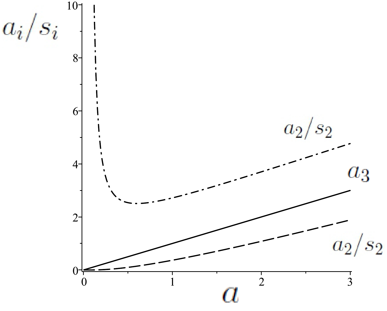
Figure 1. Profile of
a_{i} ;k=7\gamma/5 ,\xi=3\gamma/(320\pi) ,c_1=1 .\begin{aligned} a_{2\min}=c_1\cdot\left(\frac{16\pi \xi k^2}{3\gamma^3(3-2k/\gamma)}\right)^{\gamma/k}, \end{aligned}

(70) and then rises again at the end.
-
Let us consider the following borderline cases:
1. If we set
\varepsilon+\dfrac{2\gamma^2}{8\pi}=0 and\varepsilon-\dfrac{\gamma^2}{8\pi}+3\gamma\eta>0 , then\begin{aligned} \varepsilon=-1, \,\, \gamma=2\sqrt{\pi}, \,\, \eta>\frac{1}{4\sqrt{\pi}}, \,\, k<3\sqrt{\pi}, \end{aligned}

(71) and scale factors
a_{1,2} are expressed through the scale factor a:\begin{aligned}[b] a_{1,2}=&s_{1,2}\cdot a\times \exp\left\{\mp4\sqrt{\dfrac{\pi}{3k(3\sqrt{\pi}-k)}}\right.\\&\left.\cdot\sqrt{-3/2+6\eta\sqrt{\pi}+2\xi k\left(\dfrac{c_1}{a}\right)^{k/(2\sqrt{\pi})}}\right\} \end{aligned}

(72) From (59) and (71),
\begin{aligned} a=c_1\left\{\frac{2\xi k}{3|\chi|H_\infty}\left[\exp\left(\frac{kH_\infty t}{2\sqrt{\pi}}\right)-1\right]\right\}^{2\sqrt{\pi}/k },\,\, t\geq 0, \end{aligned}

(73) H_\infty=\frac{4\eta\sqrt{\pi}-1}{2|\chi|}.

In the case
2\sqrt{\pi}<k<3\sqrt{\pi} , the phase of Universe expansion without acceleration is replaced by a phase of accelerated expansion. Whenk<2\sqrt{\pi} , power-law inflation is replaced by exponential inflation over time.The anisotropic behavior of the model does not differ qualitatively from the previous one. The model becomes isotropic over time, and the scale factor
a_2 has a bounce. At the beginningt=0 , the Universe is an infinite straight line along thex_2 axis.2. If we set
\varepsilon-\dfrac{\gamma^2}{8\pi}+3\gamma\eta=0 (H_\infty= 0 ) and\varepsilon+\dfrac{2\gamma^2}{8\pi} > 0 , the scale factorsa_{1,2} are expressed through the scale factor a:\begin{aligned}[b] a_{1,2}=&s_{1,2}\cdot a\cdot\left[ \sqrt{1 +\dfrac{\nu^2 }{A^2_0}\left(\dfrac{a}{c_1}\right)^{k/\gamma}}+ \sqrt{\dfrac{\nu^2}{A^2_0}\left(\dfrac{a}{c_1}\right)^{k/\gamma}}\,\right]^{\pm\tfrac{2|\nu|\gamma}{k}}\\& \times\exp \left\{\mp\dfrac{2\gamma}{k}\cdot\sqrt{\nu^2+A^2_0\left(\dfrac{c_1}{a}\right)^{k/\gamma}}\,\right\}, \end{aligned}

(74) \begin{aligned} \nu^2\equiv\dfrac{8\pi k}{3\gamma^3}\cdot \dfrac{\varepsilon+\dfrac{2\gamma^2}{8\pi}}{3-k/\gamma}\,,\,\, A_0^2\equiv\dfrac{16\pi \xi k^2}{3\gamma^3(3-2k/\gamma)}. \end{aligned}

(75) From (58), it follows that
\begin{aligned} \frac{\sigma^2}{H^2}=\frac{\nu^2}{3}+\frac{A^2_0}{3}\left(\frac{c_1}{a}\right)^{k/\gamma}. \end{aligned}

(76) The isotropization condition (24) is not satisfied,
\begin{aligned} \frac{a_{1,2}}{a}\sim a^{\pm |\nu|}\,\,\, \text{as} \,\,\, a \rightarrow +\infty. \end{aligned}

(77) However, when
|\nu|\ll 1 , functionsa_{1,2}/a change within a narrow range,a^{\pm |\nu|}\approx \text{const} ; therefore, the anisotropy level tends to a constant low value,\begin{aligned} \left|\frac{\sigma}{H}\right|\rightarrow \frac{|\nu|}{\sqrt{3}}\ll 1\,\,\, \text{as} \,\,\, a \rightarrow +\infty. \end{aligned}

(78) A small anisotropy is allowed by observational data.
The Hubble parameter and scale factor are, respectively, given by
\begin{aligned} H=\frac{2\xi k}{3|\chi|}\left(\frac{c_1}{a}\right)^{k/\gamma}, \end{aligned}

(79) \begin{aligned} a=c_1\left[\frac{2\xi k^2}{3|\chi|\gamma}\cdot t\right]^{\gamma/k},\,\, t\geqslant 0. \end{aligned}

(80) In the case
k/\gamma<1 , we have power-law inflation. The scalar field ϕ has the time dependence\begin{aligned} \phi=\frac{1}{k}\ln\left(\frac{2\xi k^2 t}{3|\chi|\gamma}\right). \end{aligned}

(81) At early times, the model behaves in the same manner as the previous ones.
-
Let us consider the following model:
\begin{aligned} \chi=0,\,\, G=\xi\cdot\phi. \end{aligned}

(82) In this case, from Eqs. (40), (45), and (46) it follows that
\begin{aligned} \dot{\phi}=\frac{\widetilde{U}}{\alpha a^3},\,\, \widetilde{U}\equiv U(a)-C_\phi+3\gamma C_+, \end{aligned}

(83) \begin{aligned} S(a)= \frac{\beta \widetilde{U}^2}{\alpha^2a^6},\,\, N(a)=\frac{\widetilde{U}\widetilde{U}'_a}{\alpha a^6}\,, \end{aligned}

(84) where
\begin{aligned} \alpha\equiv\frac{\gamma^2}{8\pi}-\varepsilon-3\gamma\eta+2\xi,\,\,\beta\equiv\frac{2\gamma^2}{8\pi}-\frac{\varepsilon}{2}-3\gamma\eta +\xi>0. \end{aligned}

(85) Equations (47) and (48) provide the functions
\Psi(\phi) andV(\phi) :\begin{aligned}[b] \Psi&=\dfrac{a^{-1}}{3\alpha^2}\left[\left(\dfrac{\alpha}{2}-\beta\right)(\widetilde{U}^2)'_a+\dfrac{6\beta \widetilde{U}^2}{a}\right]\\&\; {=\dfrac{{\rm e}^{-2\gamma\phi}}{3c_1^2\alpha^2}\left[\left(\dfrac{\alpha}{2}-\beta\right)\gamma^{-1} [\widetilde{U}^2(a(\phi))]'_\phi+6\beta \widetilde{U}^2(a(\phi))\right],} \end{aligned}

(86) \begin{aligned}[b] V&=\dfrac{1}{6\alpha^2}\left(\beta-\dfrac{\alpha}{2}\right)\dfrac{(\widetilde{U}^2)'_a}{a^5}\\&\; {=\dfrac{\gamma^{-1}{\rm e}^{-6\gamma\phi}}{6\alpha^2 c_1^6}\left(\beta-\dfrac{\alpha}{2}\right)[\widetilde{U}^2(a(\phi))]'_\phi\,.} \end{aligned}

(87) The Hubble parameters
\sigma^2/H^2 take the form\begin{aligned} H=H_3=\frac{\gamma \widetilde{U}(a)}{\alpha a^3}, \end{aligned}

(88) \begin{aligned} H_{1,2}=H\left[ 1 \pm \sqrt{\frac{8\pi}{3\gamma^2}\left( \alpha -2\beta + \frac{6\beta}{\widetilde{U}}\int\frac{{\rm d}a \cdot \widetilde{U}}{a} + \frac{9\alpha \gamma C_+}{\widetilde{U}} \right)}\,\right], \end{aligned}

(89) \begin{aligned} \frac{\sigma^2}{H^2}=\frac{8\pi}{9\gamma^2}\left(\alpha-2\beta+ \frac{6\beta}{\widetilde{U}}\int\frac{{\rm d}a \cdot \widetilde{U}}{a}+\frac{9\alpha \gamma C_+}{\widetilde{U}}\right). \end{aligned}

(90) Choosing a simple function
\begin{aligned} U(a)=Aa^n, \,\, n>0 \end{aligned}

(91) and
C_+=C_\phi=0 , we obtain the Hubble parameter\begin{aligned} H=\frac{\gamma A}{\alpha a^{3-n}}. \end{aligned}

(92) Moreover, the condition
\begin{aligned} \frac{\gamma A}{\alpha}>0 \end{aligned}

(93) ensures Universe expansion. Therefore,
\begin{aligned} a=\left[\frac{\gamma A(3-n)}{\alpha}\cdot t\right]^{1/(3-n)}. \end{aligned}

(94) If
n<3 , thent\geq0 . In the case\begin{aligned} 2<n<3, \end{aligned}

(95) the Universe is expanding under acceleration. If
\begin{aligned} n>3, \end{aligned}

(96) then
t<0 and we obtain the Big Rip in time att=0 :\begin{aligned} a=\left[\frac{\alpha}{\gamma A(n-3)}\right]^{1/(n-3)}\cdot\left(\frac{1}{-t}\right)^{1/(n-3)},\,\, a(0)=+\infty. \end{aligned}

(97) The scalar field ϕ has the time dependence
\begin{aligned} \phi=\frac{1}{\gamma}\ln\left\{\frac{1}{c_1} \left[\frac{\gamma A(3-n)}{\alpha}\cdot t\right]^{1/(3-n)}\right\} . \end{aligned}

(98) Equations (86) and (87) provide the functions
\Psi(\phi) andV(\phi) :\begin{aligned} \Psi={\rm e}^{2(n-1)\gamma\phi}\cdot\frac{c_1^{2(n-1)}A^2}{\alpha^2} \left[2\beta+\frac{n}{3}(\alpha-2\beta)\right], \end{aligned}

(99) \begin{aligned} V={\rm e}^{(2n-6)\gamma\phi}\cdot \frac{nc_1^{2n-6}A^2\left(2\beta-\alpha\right)}{6\alpha^2}. \end{aligned}

(100) The inequalities
\begin{aligned} 2\beta+\frac{n}{3}(\alpha-2\beta)>0,\,\,2\beta-\alpha>0 \end{aligned}

(101) lead to the constraints
\Psi>0 andV>0 .The magnitude
\sigma^2/H^2 takes the form\begin{aligned} \frac{\sigma^2}{H^2}= \frac{8\pi}{3n\gamma^2}\left[2\beta+\frac{n}{3}(\alpha-2\beta)\right]=\text{const}, \end{aligned}

(102) where
\begin{aligned} \frac{8\pi}{3n\gamma^2}\left[2\beta+\frac{n}{3}(\alpha-2\beta)\right]>0. \end{aligned}

(103) The anisotropy is small,
|\sigma/H|\ll 1 , if\begin{aligned} \left|\frac{8\pi}{3n\gamma^2}\left[2\beta+\frac{n}{3}(\alpha-2\beta)\right]\right|\ll 1. \end{aligned}

(104) The Hubble parameters take the form
\begin{aligned} H_{1,2}=H\left(1\pm \sqrt{\frac{8\pi}{n\gamma^2}\left[2\beta+\frac{n}{3}(\alpha-2\beta)\right]}\,\right)\,. \end{aligned}

(105) The scale factors
a_{i} are expressed through the scale factor a:\begin{aligned} a_{1,2}=s^{\pm}_{0}\cdot a^{1\pm \sqrt{\tfrac{8\pi}{n\gamma^2}\left[2\beta+\tfrac{n}{3}(\alpha-2\beta)\right]}\,},\,\, a_3=a. \end{aligned}

(106) If condition (104) is satisfied, the Universe is close to the isotropic state:
\begin{aligned} \frac{a_{1,2}}{a}=s^{\pm}_{0}\cdot a^{\pm \sqrt{\tfrac{8\pi}{n\gamma^2}\left[2\beta+\tfrac{n}{3}(\alpha-2\beta)\right]}\,}\approx \text{const}. \end{aligned}

(107) If there is no Big Rip, the model is applicable to the era of primary inflation or late acceleration. If there is a Big Rip, the model is limited to late acceleration.
Inequalities (85), (93), (101), (103), and (104) lead to the following system:
\begin{aligned} \frac{2\gamma^2}{8\pi}-3\eta\gamma-\frac{\varepsilon}{2}+\xi>0, \end{aligned}

(108) \begin{aligned} \frac{\gamma A}{{\gamma^2}/({8\pi})-3\gamma\eta-\varepsilon+2\xi}>0, \end{aligned}

(109) \begin{aligned} \frac{\gamma^2}{8\pi}-\gamma\eta>0, \end{aligned}

(110) \begin{aligned} \frac{\gamma^2}{8\pi}(4-n)+\eta\gamma(n-6)-\varepsilon+2\xi>0, \end{aligned}

(111) \begin{aligned} \frac{8\pi}{n\gamma^2}\left[\frac{\gamma^2}{8\pi}(4-n)+\eta\gamma(n-6)-\varepsilon+2\xi\right]\ll 1. \end{aligned}

(112) Next, we provide an example of the parameters for which this system of inequalities holds. We select the parameters
\begin{aligned} \eta=0,~~ \varepsilon=1,~~ \xi=0,~~ n>2. \end{aligned}

(113) Considering (111), (112), and (113), we set
\begin{aligned} 4-n-\frac{8\pi}{\gamma^2}=\mu^2>0, \end{aligned}

(114) where
|\mu|\ll 1 . Other inequalities take the forms\begin{aligned} \frac{2\gamma^2}{8\pi}-\frac{1}{2}>0,~~\frac{\gamma A}{\dfrac{\gamma^2}{8\pi}-1}>0. \end{aligned}

(115) Two cases are allowed:
1.
\gamma A<0 . Then,1<\dfrac{8\pi}{\gamma^2}<4-n ; therefore,2<n< 3-\mu^2 . The Universe is expanding with acceleration. The Big Rip model is excluded,n<3- .2.
\gamma A>0 . Then,\dfrac{8\pi}{\gamma^2}<1 ,\dfrac{8\pi}{\gamma^2}<4-n ; therefore,3-\mu^2< n<4 . The Universe is expanding with acceleration. The Big Rip model is not excluded. -
Here, we assume
\begin{aligned} \chi\neq0,\,\, G=\xi\cdot\phi, \,\, C_\phi=C_+=0. \end{aligned}

(116) Assuming
\frac{\gamma^2}{8\pi}-\varepsilon-3\gamma\eta+2\xi=0,

\gamma>0,\,\, \dot{\phi}>0,\,\,\chi<0,\,\,U>0,

using (30) and (40), we obtain
\begin{aligned} \dot{\phi}=\left(\frac{1}{3\gamma|\chi|}\cdot\frac{U}{a^3}\right)^{1/2}, \end{aligned}

(117) \begin{aligned} H=\left(\frac{\gamma}{3|\chi|}\cdot\frac{U}{a^3}\right)^{1/2}>0, \end{aligned}

(118) that is, we obtain a model of the expanding Universe. In the case
\begin{aligned} \frac{2\gamma^2}{8\pi}-\frac{\varepsilon}{2}-3\gamma\eta+\xi=0, \end{aligned}

(119) from Eqs. (45) and (46), it follows that
\begin{aligned} S(a)=\frac{1}{(3\gamma|\chi|)^{1/2}}\cdot\left(\frac{U}{a^3}\right)^{3/2}, \end{aligned}

(120) \begin{aligned} N(a)=\left(\frac{1}{3\gamma|\chi|}\cdot\frac{U}{a^3}\right)^{1/2}\frac{U'_a}{a^3}, \end{aligned}

(121) then
\begin{aligned} \Psi=\frac{a^5}{3}\cdot\left(\frac{1}{3\gamma|\chi|}\cdot\frac{U}{a^3}\right)^{1/2}\cdot \left[\frac{U'_a}{a^3}-\frac{3}{2}\left(\frac{U}{a^3}\right)'_a\right], \end{aligned}

(122) \begin{aligned} V=\left(\frac{1}{3\gamma|\chi|}\cdot\frac{U}{a^3}\right)^{1/2} \cdot\left[\frac{U}{a^3}-\frac{a}{6}\left(\frac{U'_a}{a^3}-\frac{3}{2}\left(\frac{U}{a^3}\right)'_a\right)\right]. \end{aligned}

(123) Choosing the function
\begin{aligned} U=A^2a^{-2n+3},\,\, A>0, \end{aligned}

(124) we obtain the Hubble parameter
\begin{aligned} H=\left(\frac{\gamma }{3|\chi|}\right)^{1/2}\cdot \frac{A}{a^n}. \end{aligned}

(125) Therefore,
\begin{aligned} a=\left(\sqrt{\frac{\gamma}{3|\chi|}}\cdot nA\cdot t\right)^{1/n}. \end{aligned}

(126) If
n>0 , thent\geq0 . In the case0<n<1 , the Universe is expanding under acceleration. Ifn<0 , thent<0 and we achieve the Big Rip in time att=0 :\begin{aligned} a=\left[\sqrt{\frac{\gamma}{3|\chi|}}\cdot |n|A\right]^{-1/|n|}\cdot\left(\frac{1}{-t}\right)^{1/|n|},\,\, a(0)=+\infty. \end{aligned}

(127) The scalar field ϕ has the time dependence
\begin{aligned} \phi=\frac{1}{\gamma}\ln\left\{\frac{1}{c_1} \left(\sqrt{\frac{\gamma}{3|\chi|}}\cdot nA\cdot t\right)^{1/n}\right\} . \end{aligned}

(128) Equations (34), (122), and (123) provide the functions
\Psi(\phi) andV(\phi) :\begin{aligned} V=\frac{(3-n)A^{3}}{6(3\gamma|\chi|)^{1/2}a^{3n}}=\frac{(3-n)A^{3}}{6(3\gamma|\chi|)^{1/2}c_1^{3n}}\cdot {\rm e}^{-3n\gamma\phi}, \end{aligned}

(129) \begin{aligned} \Psi=\frac{\left(3+n\right)A^{3}a^{4-3n}}{3(3\gamma|\chi|)^{1/2}}= \frac{\left(3+n\right)A^{3}c_1^{4-3n}}{3(3\gamma|\chi|)^{1/2}}\cdot {\rm e}^{(4-3n)\gamma\phi}. \end{aligned}

(130) The inequalities
\begin{aligned} -3<n<3 \end{aligned}

(131) lead to the constraints
\Psi>0 andV>0 .The Hubble parameters take the form
\begin{aligned} H_{1,2}=H\left[1\pm\sqrt{\frac{8\pi |\chi|^{1/2}A(3+n)}{3^{1/2}\gamma^{3/2}(3-2n)}}\cdot\frac{1}{a^{n/2}}\,\right], \end{aligned}

(132) where a new requirement arises,
n<3/2 . The scale factorsa_{i} are expressed through the scale factor a:\begin{aligned} a_{1,2}=s_{1,2}\cdot a\cdot\exp\left[\mp\frac{2}{na^{n/2}} \cdot\sqrt{\frac{8\pi |\chi|^{1/2}A(3+n)}{3^{1/2}\gamma^{3/2}(3-2n)}}\,\right]. \end{aligned}

(133) The model isotropization condition is satisfied for
n>0 :\begin{aligned}[b] \frac{a_{1,2}}{a}=&s_{1,2}\cdot\exp\left[\mp\frac{2}{na^{n/2}} \cdot\sqrt{\frac{8\pi |\chi|^{1/2}A(3+n)}{3^{1/2}\gamma^{3/2}(3-2n)}}\,\right]\\&\rightarrow \text{const} \,\,\, \text{as} \,\,\, a \rightarrow +\infty. \end{aligned}

(134) Because
n>0 , the Big Rip is excluded. The anisotropic properties of model (133) are similar to those of model (69). The functiona_2 falls from a greater value at the beginning, bounces to the minimum value\begin{aligned} a_{2{\rm min}}=\left(\frac{8\pi |\chi|^{1/2}A(3+n)}{3^{1/2}\gamma^{3/2}(3-2n)}\right)^{1/n} \end{aligned}

(135) and then rises again at the end. At the beginning,
t=0 , the Universe is an infinite straight line along thex_2 axis:a_1(0)=a_3(0)=0 ,a_2(0) =+\infty . The model can be applied to the early Universe before the end of primary inflation. -
We construct anisotropic models in BI for a subclass of HG:
\begin{aligned}[b] G_4&=1/(16\pi),\,\,G_2=\varepsilon X-V(\phi),\\ G_5&=-\dfrac{1}{32\pi \gamma X},\,\, G_3=\dfrac{\eta}{2}\ln\dfrac{X}{C}+\chi\sqrt{2X}+G(\phi). \end{aligned}

(136) with the non-minimal interaction by the law
f^2(\phi)F_{\mu\nu}F^{\mu\nu} .Using the reconstruction method, we present functions
\Psi(\phi)=q_m^2f^2(\phi) andV(\phi) , for which the isotropization criterion\lim\limits_{a\rightarrow \infty} a_i/a=\text{const} is satisfied.The function
G_5\sim 1/X results in the possibility of an anisotropic bounce. At the beginning,t=0 , the Universe is an infinite straight line along thex_2 axis:a_1(0)= a_3(0)=0 ,a_2(0) =+\infty .Combinations of the parameters
\varepsilon ,\gamma ,\eta ,\chi , andG(\phi) allow for different possibilities for Universe development: power-law inflation, exponential inflation, the Big Rip, and two-phase expansion. In all cases, the anisotropy behavior is acceptable.In conclusion, we find a method of obtaining exact solutions for a large subclass of HG with an electromagnetic field.
Isotropization of the magnetic universe in Horndeski theory with G3(X,ϕ) and G5(X)
- Received Date: 2024-05-12
- Available Online: 2024-11-15
Abstract: We study the isotropization process of Bianchi-I space-times in Horndeski theory with


 DownLoad: