-
At high energy, the scattering process with a hadron actually involves the internal constituents, namely the quarks and the gluons, which are commonly called the partons. Thus, to obtain the cross-sections of these scattering processes, information from partons should be acquired. Generally, partons are described using the parton distribution function (PDF), which defines the probability that the parton carries a certain momentum fraction of the hadron momentum. Therefore, the determination of the PDFs of hadrons has remained an important project in hadron physics.
The PDF is difficult to predict in theory as it involves non-perturbative quantum chromodynamics (QCD). Traditionally, only the first few moments of a PDF are calculated and then methods are adopted to reconstruct the PDF [1−7]. Although the new methods that can directly obtain the PDF have been proposed in recent years [8−12], many problems continue to occur, such as excessive error and limited computable regions. The reconstruction of the PDF with the finite moments is a problem that needs to be frequently addressed. Accordingly, various methods have been developed. However, these methods require assumption of the functional form of the PDF in advance and then use moments to determine the parameters, ultimately completing the reconstruction. The presupposition of the PDF form inevitably includes some artificial choices, providing insufficient reconstruction results.
In this study, we propose a new reconstruction method for the symmetric PDF of the pion to avoid the impact of artificial choice. This method obtains the PDF by maximizing entropy under moment constraints, without the need to introduce any artificial presets regarding the PDF. This paper is organized as follows: Section II provides details on the new reconstruction method, including the cases of precise moments and moments with errors. Section III presents the series of calculation results, including validity test, reconstruction efficiency assessment based on artificial inputs, and the results corresponding to real inputs. Finally, a summary is presented in Sec. IV.
-
The maximum entropy method is utilized to determine the distribution function
$ f(x) $ , which is a mature idea that has been practiced multiple times [13−15]. The Shannon entropy of the distribution function$ f(x) $ is defined as follows:$ S=-\int_{0}^1 f(x)\log f(x){\rm d}x . $

(1) If the system has no constraints, it will produce a constant distribution function, which is the principle of equal a priori probabilities. However, the distribution of partons requires several constraints to be considered. These constraints for the pion at the hadron scale can be mathematically expressed as follows:
$ \int _{0}^{1}f(x){\rm d}x=1, $

(2) $ f(x)=f(1-x), $

(3) $ \int _{0}^{1}x^i f(x){\rm d}x=\mu_{i}. $

(4) We define a Lagrange function L to describe the system, so that entropy and all the constraints can be combined, as follows:
$ L = S+\sum\limits_{i=0}^{m}\lambda_{i}\Delta_i, $

(5) where
$ \lambda_i $ are unknown coefficients, and$ \Delta_i = \int_0^1x^if(x){\rm d}x - \mu_i^{\rm prior} $

(6) where
$ \mu_i^{\rm prior} $ are the prior informations or constraints given by the first principle theory.Considering the challenges of obtaining an analytical solution for the distribution function, it is often beneficial to employ an approximate distribution function with undetermined coefficients. The larger the number of coefficients included, the higher the flexibility of the distribution function. Additionally, regarding the system's symmetry, we selected a suitable basis set, given by
$ f(x)=\sum\limits_{k=1}^{n}a_{k}\sin{(2k-1)}\pi x . $

(7) If the system function has reached its maximum point, the derivation of the Lagrange function should be equal to zero:
$ \frac{\partial L}{\partial\lambda_i}=0,\quad \frac{\partial L}{\partial a_{j}}=0. $

(8) This reconstruction has thus been converted so that only the derivation equations need to be solved. However, determining the analytical solutions to these complex equations is challenging. To resolve this, we adopted the self-consistent field (SCF) method, originally introduced by Hartree for solving multiple-electron systems [16]. This method is valuable for seeking the steady status of a complex system with constraints and one system function. Starting with initial values, the SCF process iteratively finds nearby steady solutions. The SCF process can be described using the recurrence equation:
$ \begin{array}{*{20}{l}} \begin{bmatrix} \lambda_0\\ \vdots\\ \lambda_m\\ a_1\\ \vdots\\ a_n \end{bmatrix}_{k+1}= \begin{bmatrix} \lambda_0\\ \vdots\\ \lambda_m\\ a_1\\ \vdots\\ a_n \end{bmatrix}_{k}+\xi{\boldsymbol{H}}^{-1} \begin{bmatrix} -\Delta_0\\ \vdots \\ -\Delta_m\\ -\dfrac{\partial L}{\partial a_1} \\ \vdots\\ -\dfrac{\partial L}{\partial a_n} \end{bmatrix}, \end{array} $

(9) In this equation,
$ {\boldsymbol{H}} $ represents the bordered Hessian matrix of Shannon entropy S. Specifically, it can be represented as$ \begin{array}{*{20}{l}} {\boldsymbol{H}} = \begin{bmatrix} 0&\cdots&0& \dfrac{\partial \Delta_0}{\partial a_1}&\cdots & \dfrac{\partial \Delta_m}{\partial a_1} \\ \vdots&\ddots &\vdots &\vdots & \ddots &\vdots \\ 0&\cdots&0 &\dfrac{\partial \Delta_0}{\partial a_n}&\cdots & \dfrac{\partial \Delta_m}{\partial a_n} \\ \dfrac{\partial \Delta_0}{\partial a_1}&\cdots &\dfrac{\partial \Delta_0}{\partial a_n}&\dfrac{\partial^2 L}{\partial a_1\partial a_1} &\cdots &\dfrac{\partial^2 L}{\partial a_n\partial a_1} \\ \vdots&\ddots&\vdots&\vdots&\ddots&\vdots \\ \dfrac{\partial \Delta_m}{\partial a_1}&\cdots &\dfrac{\partial \Delta_m}{\partial a_n}&\dfrac{\partial^2 L}{\partial a_1\partial a_n} &\cdots &\dfrac{\partial^2 L}{\partial a_n\partial a_n} \end{bmatrix}, \end{array} $

(10) where
$ \frac{\partial \Delta_m}{\partial a_k} = \int_0^1 x^m \sin{(2k-1) \pi x} {\rm d}x, $

(11) $ \frac{\partial^2 L}{\partial a_j\partial a_k} = -\int_0^1 \frac{(\sin{(2j-1) \pi x})( \sin{(2k-1) \pi x})}{f(x)} {\rm d}x. $

(12) In this equation, ξ represents the step size. A larger ξ leads to a faster convergence process but may compromise program stability when the initial values are inadequate. For all calculations in this paper, the default value of
$ \xi=1 $ is used. Moreover, we set the iterative tolerance to$ 10^{-5} $ , which provides sufficient accuracy for our calculations.After obtaining the coefficients, a reasonableness test is necessary to ensure that the result represents the local maximum point of entropy. For this purpose, the bordered Hessian matrix must satisfy a sufficient condition: the leading principal minors starting from
$ 2m+1 $ must alternate in sign, with the smallest one having the sign of$ (-1)^{m+1} $ .In conclusion, this SCF method contains five steps:
● Guess the initial values of the coefficient array;
● Obtain the Hessian matrix (integration is calculated by the grid point method);
● Calculate the inverse of the Hessian matrix and update the coefficient array;
● Determine whether the variation of the Lagrange function is less than the preset tolerance
$ 10^{-5} $ . If not, go back to the second step;● Reasonableness test. If the test fails, repeat the process with the new initial value.
-
The calculated results of the moment of the PDF obtained by QCD are always accompanied by errors, represented as
$ \mu_i \pm \sigma_i $ . Consequently, using the simple Lagrange functions to address these constraints is insufficient, as they impose excessively strict conditions. Therefore, it is necessary to relax the moment constraints. One approach to achieving this is by replacing the original constraint terms with a relaxation function. In our study, we employ the Gaussian-shaped function as this relaxation function:$ \lambda_i\Delta_i\to E_i(f)=\frac{1}{\sqrt{2\pi}\sigma_i}\exp{\left(-\frac{\Delta_i^2}{2\sigma_i^2}\right)}\ (i=1,2,\dots,m). $

(13) Notably, the above replacement starts from
$ i=1 $ as$ \Delta_0 $ , which serves as the normalization factor, is known to be completely accurate. The peak of the Gaussian-shaped function corresponds to the center of the error bar, with its value gradually increasing as$ \Delta_i $ approaches zero. Additionally, as$ \sigma_i $ increases to represent larger errors, the curve becomes flatter. Consequently, the constraint of moments is weakened in proportion to its uncertainty. Considering these properties, our replacement is a reasonable approach.Introducing this Gaussian shape function, the new Lagrange function is corrected as follows:
$ L' = S + \lambda_0 \Delta_0 + \beta \sum\limits_{i=1}^m E_i(f), $

(14) where the coefficient β represents the strength of the constraints. By adjusting the value of β, the model can effectively control the trade-off between maximizing the entropy and satisfying the moment constraints. A higher value of β emphasizes the importance of meeting the constraints, resulting in a distribution that closely aligns with the specified moments. Conversely, a lower value of β places more emphasis on maximizing the entropy, allowing for a distribution that may deviate slightly from the constraints. Correspondingly, the SCF method changes by replacing L with
$ L' $ . -
Within our model, two parameters, i.e., the term number of the basis set and the size of the grid point, are determined through comparison with the analytical solution. In scenarios where the distribution is constrained solely by the second-order moment, the PDF can be ascertained by the variational approach. This approach yields a Gaussian function as the analytical solution. Specifically, when the second moment
$ \mu_2=0.3 $ , the Gaussian function is represented as follows, with an associated entropy of$ -0.114 $ :$ \begin{array}{*{20}{l}} f(x) = 1.63\exp{\left(-7.5(x-0.5)^2\right)}. \end{array} $

(15) For the same situation, we calculate entropy using the SCF method with various parameters and then compare these results with the analytical results. The relative error obtained from the comparison is visualized in Fig. 1.
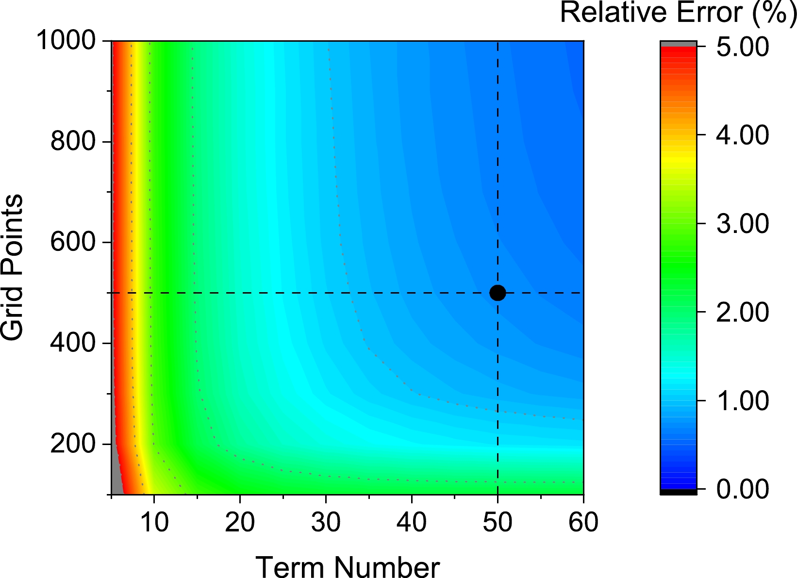
Figure 1. (color online) Relative errors of entropy by the SCF method with various parameters. Gray dotted lines signify integer percents, and the black point signifies parameters utilized in our reconstruction.
Based on the analysis of entropy, our approach demonstrates a high level of reliability. Opting for a denser grid and a larger basis set generally yields more accurate results but at the expense of heightened computational time. Specifically, the time complexity of the term number and the grid size are
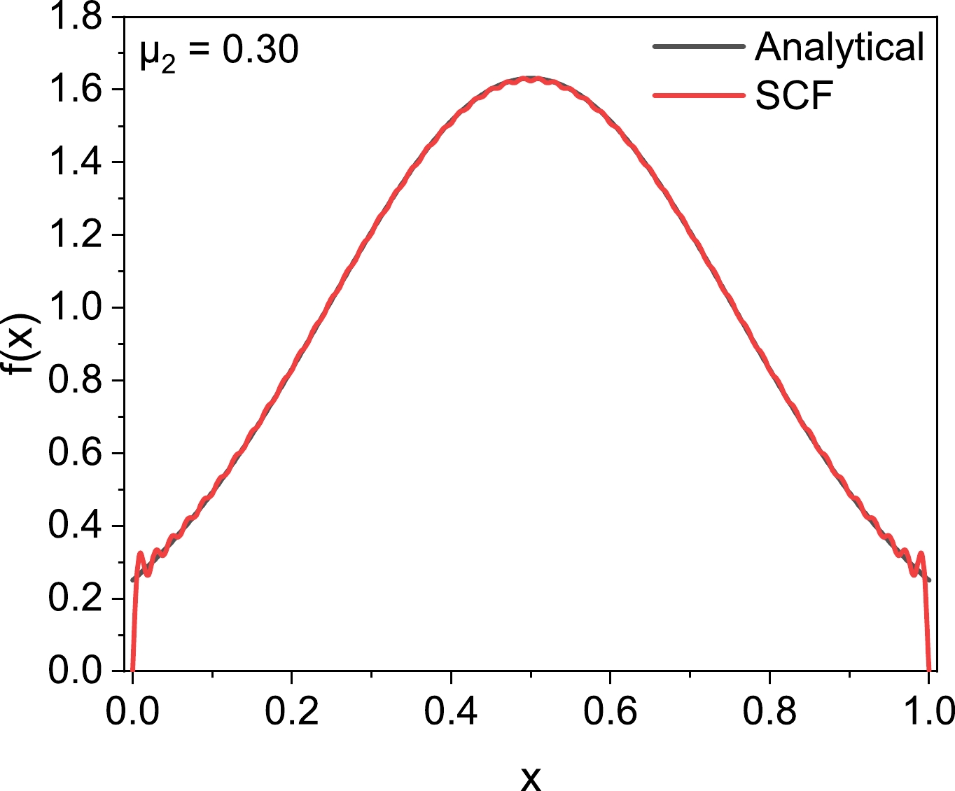
$ O(N^3) $ and$ O(N) $ , respectively. Consequently, striking the right balance between time efficiency and accuracy is of utmost importance. Given our available computational resources, all calculations presented in this paper were conducted employing 50 terms and 500 points.The analysis discussed above is exclusively based on entropy, which only carries partial information about distribution. Therefore, a more nuanced comparison is necessary. To elucidate the deviation at each data point, we compare the SCF result using the aforementioned parameters with the analytical result, which is shown in Fig. 2.
It is evident that the curve from the SCF method closely aligns with the Gaussian distribution derived through the variational approach. Notably, the SCF method produces the anticipated outcome within the majority of the function's range, indicating that our method is sufficiently reliable. Nevertheless, slight oscillations can be observed at the tails of the distribution function. These oscillations primarily arise due to the nature of the basis set.
-
This section concerns discussion of a model that holds physical significance. Our objective is to assess the effectiveness of reconstruction under different numbers of constraints. The symmetric function presented below is a widely used form for characterizing the distribution of partons:
$ \begin{array}{*{20}{l}} f(x)=N_{\rho}\log(1+x^2(1-x)^2/\rho^2), \end{array} $

(16) where
$ N_{\rho} $ is the normalization constant.This function is effective enough to describe PDF by adjusting ρ. Notably, there exists a unique correspondence between the parameters ρ and
$ \mu_2 $ within this distribution; for example, when$ \mu_2 $ equals$ 0.3 $ , the corresponding value of ρ is$ 0.0658 $ . Considering the specific physical meanings of$ \mu_2 $ , in this section, we apply$ \mu_2 $ to represent different functions.Subsequently, to show the efficiency of reconstruction under different numbers of constraints, we use the first few moments corresponding to
$ \mu_2=0.3 $ as constraints to attempt to reconstruct the distribution. The resulting distribution functions and entropy are displayed in Figs. 3 and 4, respectively. Only even numbers are considered since odd-order moments are not independent because of the symmetry.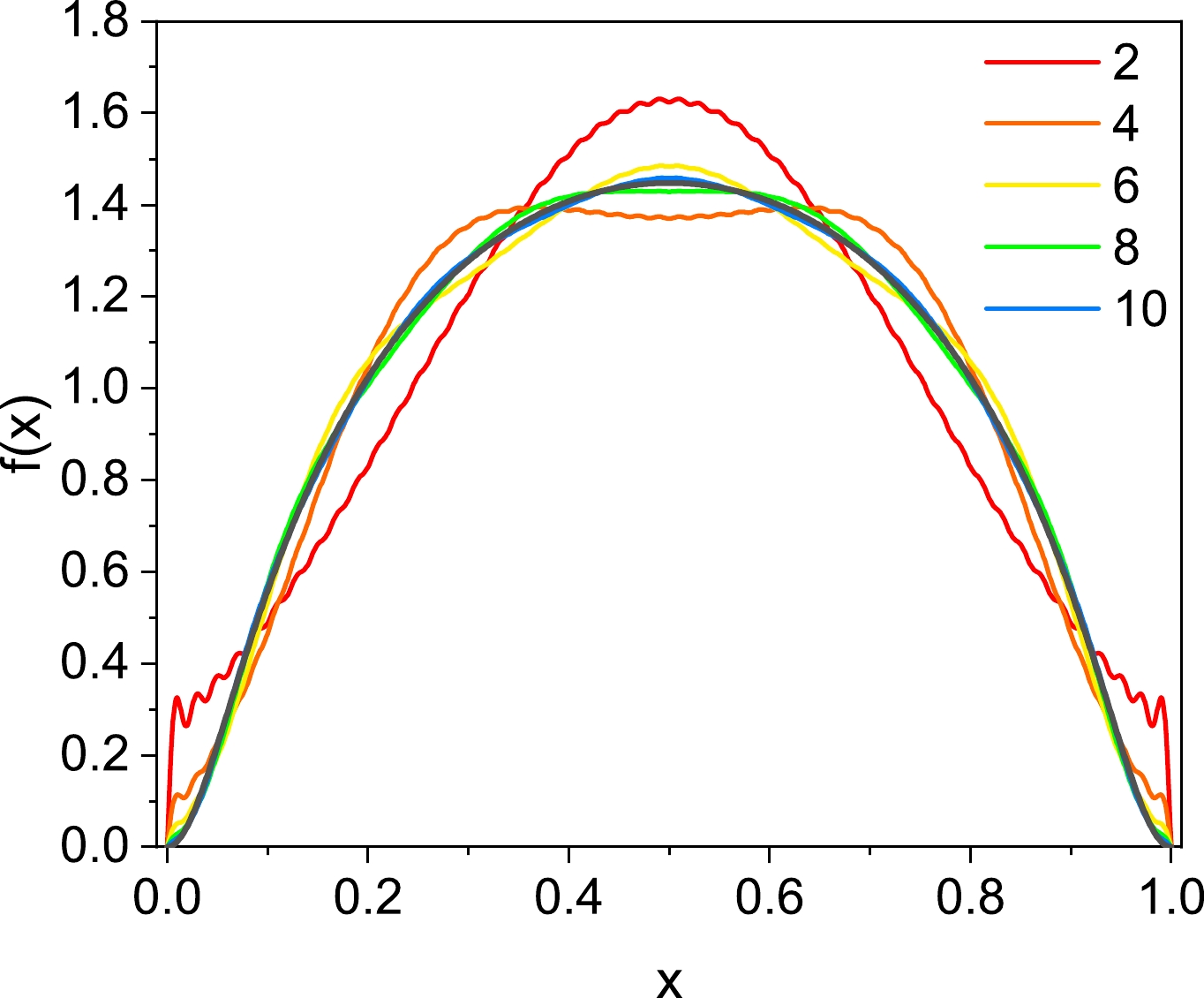
Figure 3. (color online) Variation in reconstruction results under different numbers of constraints. The black curve represents the target symmetric function.
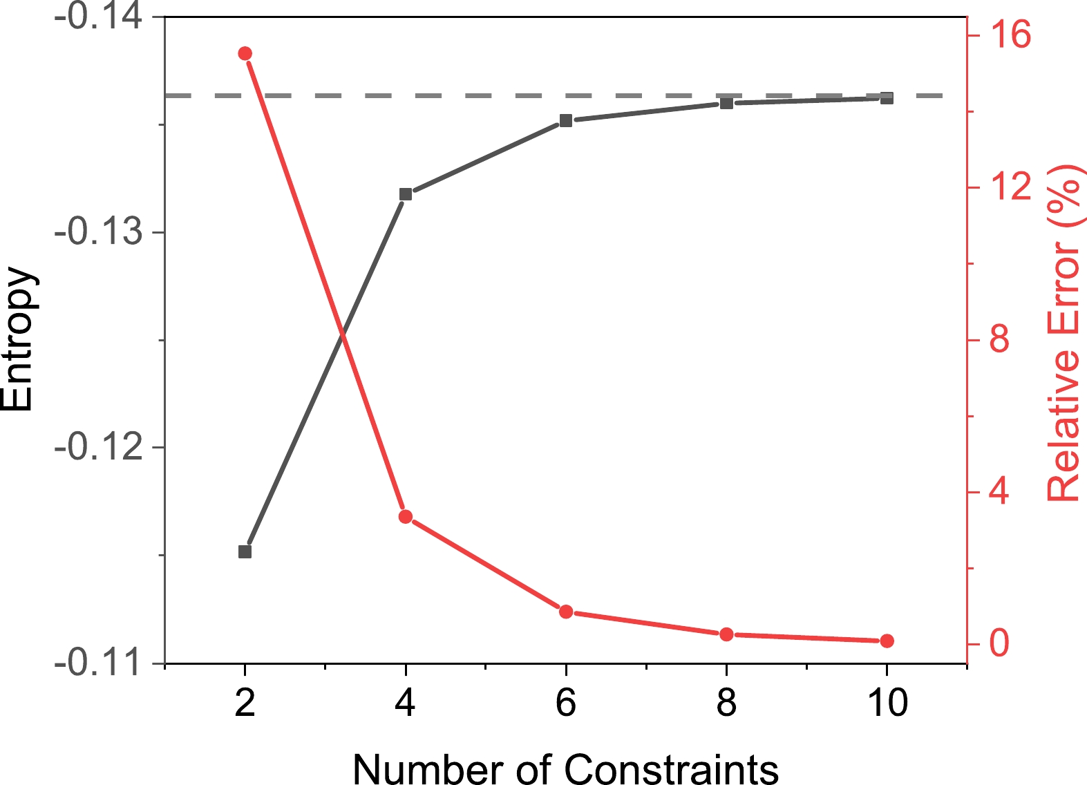
Figure 4. (color online) Variation in entropy under different numbers of constraints. The entropy and relative error are represented by the black and red curves, respectively. The gray dashed line represents the entropy of the target symmetric function.
Figures 3 and 4 unmistakably illustrate that as additional constraints are integrated, the outcomes progressively approach the sought-after symmetric function, i.e., the efficiency of reconstruction improves. Importantly, it is apparent that with a minimum of six moment constraints, the precision of the reconstruction reaches a high level, with an error margin of approximately
$ 1 $ %. Notably, employing ten constraints yields a considerably robust and accurate reconstruction. Therefore, reconstruction with at least six constraints is suggested for a reliable result.The comprehensive analysis thus far exclusively concerns the scenario wherein
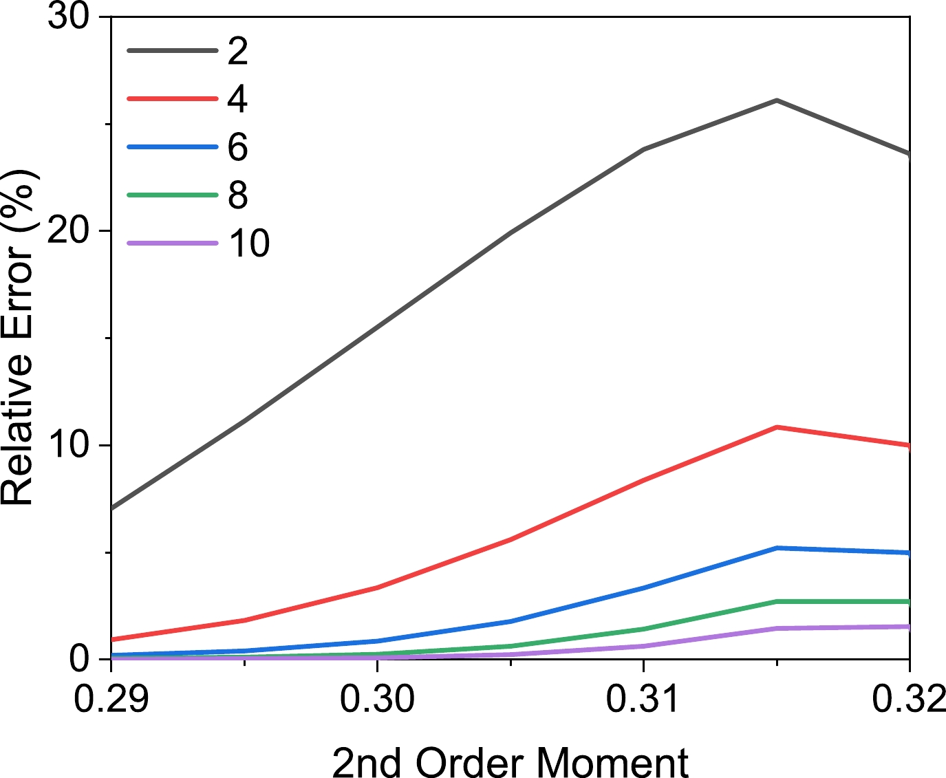
$ \mu_2 $ is equal to$ 0.3 $ . Therefore, the calculations must be extended across a spectrum of$ \mu_2 $ values to validate the robustness of our previous conclusions. Figure 5 presents the relative errors of entropy for varying$ \mu_2 $ values ranging from$ 0.29 $ to$ 0.32 $ . This scope comprehensively covers the possible scenarios for the PDF to confirm the generalizability of the earlier-drawn conclusions.The insights provided by Fig. 5 indicate that relative errors exhibit an increasing trend as the second-order moment increases. However, for the six constraints case, the relative error remains confined within a threshold of
$ 5\ $ %. This level of variability has been found to be satisfactory for a significant proportion of reconstruction tasks. Therefore, a minimum of six constraints provides the necessary foundation for achieving reliable and accurate reconstructions. -
This section outlines the reconstruction based on real data with error bars. The first six moments of the pion valence-quark distribution are provided using lattice QCD in Ref. [17]. However, these data are all at
$ 5.2 $ GeV, and the PDF at this scale is not symmetric. Therefore, we altered these data to the hadron scale according to the method in Refs. [18, 19], and the results are displayed in Table 1.Order 1 2 3 4 5 6 Moment $ 0.5 $ 

$ 0.29(3) $ 

$ 0.19(5) $ 

$ 0.14(5) $ 

$ 0.10(5) $ 

$ 0.08(4) $ 

Table 1. Data for the first six moments
To select an appropriate value for β, it is crucial to understand how the entropy curve behaves under different β settings. Figure 6 represents the changes in entropy with varying values of β.
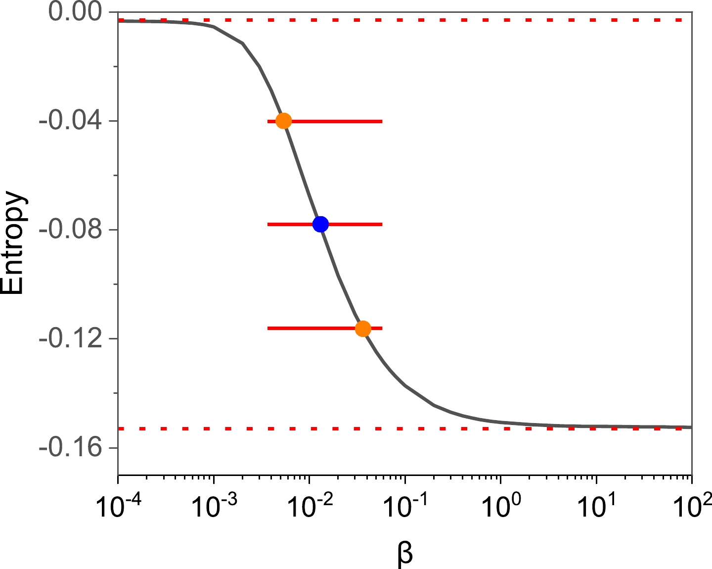
Figure 6. (color online) Variations in entropy values as β changes. The axis is converted to a logarithmic scale. Red dashed lines serve as asymptotes, while the blue and orange dots correspond to the median and boundaries of the error range of β, respectively.
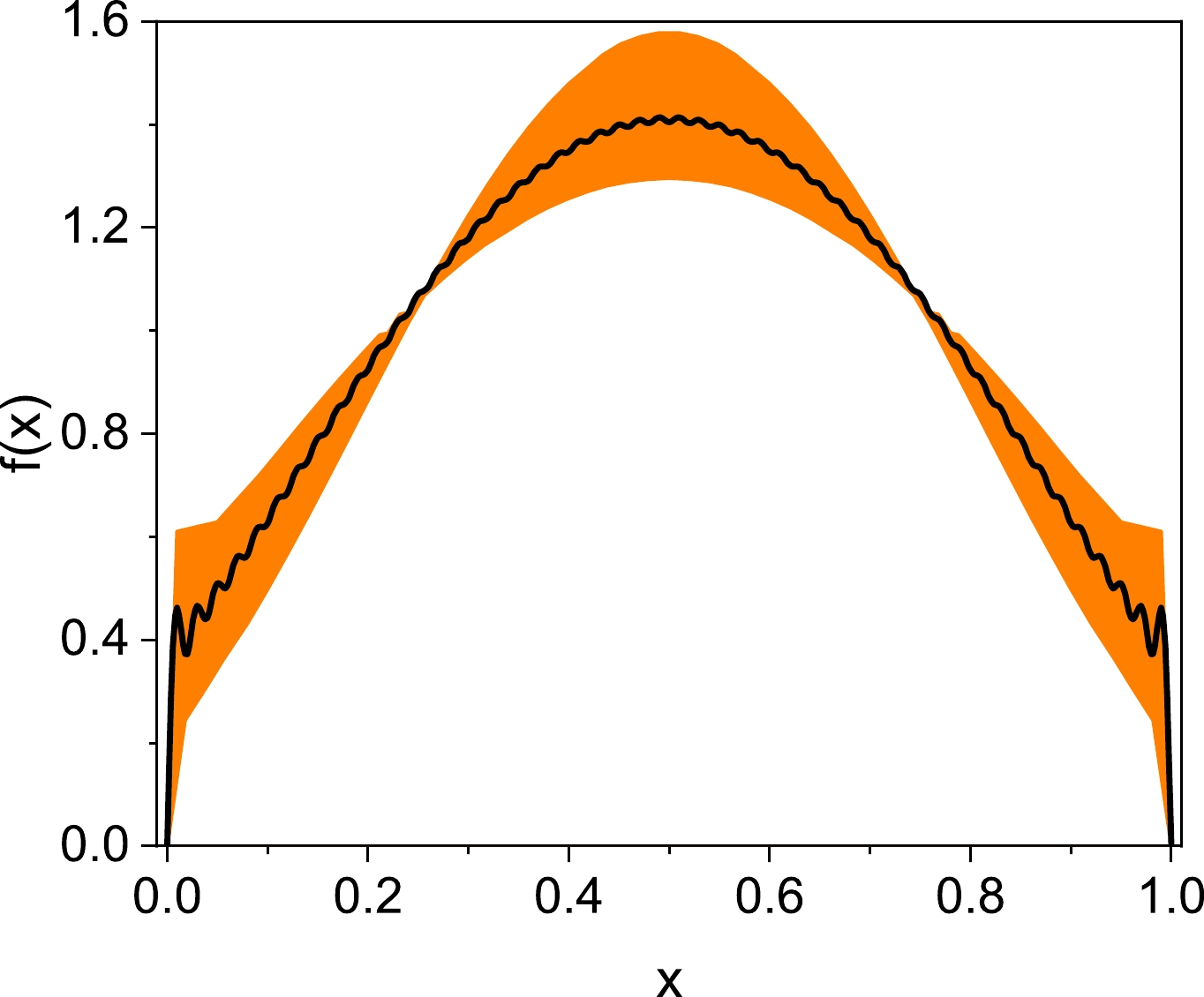
In Fig. 6, we observe a significant trend: as β increases, there is a consistent decrease in entropy. At both extremes, we observe a convergence toward two distinct values. One corresponds to a state where maximum entropy prevails, while the other represents a situation where constraints are rigorously enforced. This observation aligns seamlessly with our earlier discussions. As a consequence, it is reasonable to infer that the ideal value for β lies somewhere between these two extremes. A straightforward approach involves selecting the midpoint between these extremes as the ideal value for β. To quantify our uncertainty, we recommend defining an error range by dividing the entropy range into four equal parts and designating the two central segments as the error range. This distribution function and its associated error range are described in Fig. 7. Additionally, Fig. 8 presents a comparison between the lattice input and moment error range of the reconstruction result.
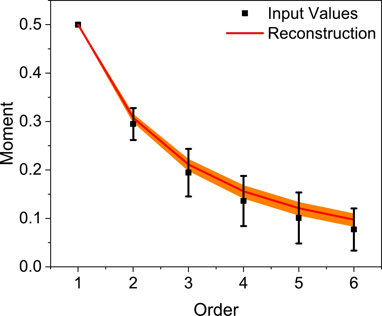
Figure 8. (color online) Comparison between the lattice input and moment error range of the reconstruction result.
As can be seen in Fig. 7, the reconstruction result is outstanding, closely mirroring the findings reported in prior research as detailed in Ref. [20]. This striking similarity underscores the robustness and consistency of our reconstruction method. Moreover, Fig. 8 clearly shows that the error range of our reconstruction is well within compatibility bounds with the lattice input. However, it is important to note that the error range of the current reconstruction consistently lies slightly above the lattice input, particularly for higher-order moments, where a more noticeable deviation is observed.
In conclusion, the effectiveness and reliability of the proposed reconstruction method have been proven in this work. However, a more precise method for selecting the optimal β value requires further investigation and research.
-
In this study, we combined the first few moments and entropy as constraints to define the Lagrange function and numerically reconstruct the PDF at the maximum point of the Lagrange function. To include the error in calculating moments with QCD, we replaced the original moment constraints with Gaussian-shaped functions to soften the constraints. Accordingly, the result appears more natural and convincing than the methods that presuppose the function form of PDF artificially.
Furthermore, we comprehensively evaluated the convergence and reconstruction efficiency of the proposed method of reconstructing PDF; the results show that our method is reasonable. As the number of moments entered increases, the results become more accurate, and high-quality reconstruction is achieved using only the first six moments as input. Moreover, a set of lattice QCD results were selected regarding moments in Ref. [17] as input to reconstruct the PDF. Finally, an excellent reconstruction result was produced and provide a reasonable error band.
Although reasonable and reliable results are obtained, using this PDF reconstruction method, which avoids artificial selection, the method can be further developed. For the input with error, we can multiply each
$ \Delta_i $ by$ \beta_i $ , which can increase the accuracy of the calculation but also increases the difficulty of the calculation. For the asymmetric case, the base set can be replaced, but this leads to greater computational complexity and potential convergence difficulty. It is hoped that this work can promote the research of PDF reconstruction in the field of hadron structure.
Reconstructing parton distribution function based on maximum entropy method
- Received Date: 2023-09-06
- Available Online: 2024-03-15
Abstract: A new method based on the maximum entropy principle for reconstructing the parton distribution function (PDF) from moments is proposed. Unlike traditional methods, the new method does not require any artificial assumptions. For the case of moments with errors, we introduce Gaussian functions to soften the constraints of moments. Through a series of tests, the effectiveness and reconstruction efficiency of this new method are evaluated comprehensively, demonstrating that this method is reasonable and can achieve high-quality reconstruction with at least the first six moments as input. Finally, we select a set of lattice quantum chromodynamics (QCD) results regarding moments as input and provide reasonable reconstruction results for the pion.


 Abstract
 HTML
HTML Reference
 Related
 PDF
PDF




 DownLoad: