Molecular states in ${\boldsymbol{D_s^{(*)+}} \boldsymbol{\Xi_c^{(',*)}}}$ systems

The study of multiquark states began even before the birth of quantum chromodynamics (QCD) and accelerated with the development of QCD. It is speculated that other than the well-known $qqq$-baryons and $q\bar q$-mesons [1, 2], there may be multiquark states, glueballs, and quark-gluon hybrids in the quark model notation, which are collectively known as exotic hadrons. Multiquark states can be categorized into tetraquark states ($qq\bar q \bar q$), pentaquark states ($qqq q\bar q$), and so on. The study of multiquark states, especially the internal grouping of quarks (i.e., compact or molecular configuration), plays a crucial role in understanding low energy QCD.

In the past two decades, many candidates of exotic tetraquark and pentaquark states have been observed in experiments (see Refs. [3−20] for recent reviews on the experimental and theoretical status of exotic hadrons). An intriguing fact is that most of them are located close to the thresholds of a pair of hadrons to which they can couple. This property can be explained by an S-wave attraction between the relevant hadron pair [21], which naturally leads to their hadronic molecule interpretation (as reviewed in Refs. [3, 8, 14, 17, 19, 20]). In the hadronic molecular picture, several of them can be interpreted as the loosely bound states of two hadrons via the strong interaction parameterized by light meson exchange at low energy. The validity of the hadronic molecular picture is also reflected by the successful quantitative predictions of some exotic states in early theoretical studies on hadron-hadron interactions (see, e.g., Refs. [22−30]).

The pentaquark states $P_c(4450)$ and $P_c(4380)$ were observed by the LHCb collaboration [31] in 2015. In the updated measurement [32], the $P_c(4450)$ signal split into two narrower peaks, $P_c(4440)$ and $P_c(4457)$; however, there was no clear evidence for the previous broad $P_c(4380)$ ¹. Meanwhile, a new narrow resonance $P_c(4312)$ showed up. Several models have been applied to understand the structures of these states, and the $\bar D^{(*)} \Sigma_c^{(*)}$ molecular explanation, which appeared in Refs. [23−28, 30, 34] even before LHCb observations, stands out because it can explain the three states simultaneously (see, e.g., Refs. [35−38]). The success of the hadronic molecule picture for the $P_c$ states prompted the extension of $\bar D^{(*)} \Sigma_c^{(*)}$ systems to their SU(3) flavor partners with hidden-charm (double-)strangeness channels [39−48]. Recently, two $P_{cs}$ states were reported by the LHCb collaboration, $P_{cs}(4459)$ [49] and $P_{cs}(4338)$ [50], which are perfect candidates of the $\bar D^*\Xi_c$ and $\bar D\Xi_c$ molecules, respectively (see, e.g., Refs. [17, 51−64]).

Last year, the LHCb collaboration announced the discovery of a double-charm exotic state, $T_{cc}^+(3985)$, which reveals itself as a high-significance peaking structure in the $D^0D^0\pi^+$ invariant mass distribution just below the nominal $D^{*+}D^0$ threshold [65, 66]. This observation motivated numerous studies on double-charm tetraquark states, and $T_{cc}^+(3985)$ is a perfect candidate of the isoscalar $1^+ DD^*$ molecule (see, e.g., Refs. [67−76]).

It is well known that the interaction between a pair of hadrons can be effectively described by light meson (pseudoscalar and vector) exchange. Resonance saturation has been known to effectively approximate the low-energy constants (LECs) in the higher order Lagrangians of chiral perturbation theory [77, 78], and it turns out that whenever vector mesons contribute, they dominate the numerical values of LECs at the scale around the ρ-meson mass, which is referred to as the modern version of vector meson dominance. Under this vector meson dominance assumption, it can be easily verified that $D^{(*)}\Sigma_{c}^{(*)}$ systems are more attractive than the corresponding $\bar D^{(*)}\Sigma_{c}^{(*)}$ systems [19], the latter of which corresponds to the experimentally observed $P_c$ states. Such observation leads to the predictions of more deeply bound double-charm pentaquarks in the molecular scenario [19, 79−84].

In this study, we extend the investigation of double-charm pentaquarks to systems with hidden-strangeness. Specifically, we explore the light-meson-exchange ($\phi,\sigma,\eta$) interactions in $D_s^{+}\Xi_c$-$D_s^{+}\Xi_c^{'}$-$D_s^{*+}\Xi_c$-$D_s^{+}\Xi_c^{*}$-$D_s^{*+}\Xi_c^{'}$-$D_s^{*+}\Xi_c^{*}$ systems and search for possible poles near the corresponding thresholds. In Sec. II, we introduce our theoretical framework, including the involved channels, the relevant Lagrangian satisfying heavy quark spin symmetry (HQSS) and SU(3) flavor symmetry, and the light-meson-exchange potentials in terms of known parameters. In Sec. III, we present the numerical results and discussions. Finally, we provide a brief summary in Sec. IV.

The one-boson-exchange (OBE) potential model has been successful in interpreting the formation mechanisms of pentaquarks [38, 85−88]. In this study, we also use the OBE potentials of the $D_s^{(*)+}\Xi_c$, $D_s^{(*)+}\Xi_c^{'}$, and $D_s^{(*)+}\Xi_c^{*}$ systems to investigate the possibility of double-charm pentaquarks with hidden-strangeness in the molecular picture.

In our analysis, we focus on hadronic molecules with spin-parities $J^P=1/2^-,3/2^-$, and $5/2^-$ in the $D_s^{(*)+}\Xi_c$, $D_s^{(*)+}\Xi_c^{'}$, and $D_s^{(*)+}\Xi_c^{*}$ systems because the negative-parity states of these channels can be coupled in the S-wave, which is usually the most important partial wave component in a hadronic molecule. The thresholds and spin-orbital wave functions of these channels are listed in Table 1, where the notation $^{2S+1}L_J$ is used to identify various partial waves. S, L, and J denote the total spin, orbital and total angular momenta, respectively. The state in the partial wave $^{2S+1}L_J$ with a certain z-direction projection m can be explicitly written as

Channels	$D_s^+\Xi_c$	$D_s^{+}\Xi_c^{'}$	$D_s^{*+}\Xi_c$	$D_s^+\Xi_c^*$	$D_s^{*+}\Xi_c^{'}$	$D_s^{*+}\Xi_c^*$
Threshold/MeV	$4437.76$	$4547.14$	$4581.62$	$4614.31$	$4691.00$	$4758.17$
$J^P=1/2^-$	$|^2S_{1/2}\rangle$	$|^2S_{1/2}\rangle$	$\begin{pmatrix}|^2S_{1/2}\rangle\\ |^4D_{1/2}\rangle\end{pmatrix}$	$|^4D_{1/2}\rangle$	$\begin{pmatrix}|^2S_{1/2}\rangle\\ |^4D_{1/2}\rangle\end{pmatrix}$	$\begin{pmatrix}|^2S_{1/2}\rangle\\ |^4D_{1/2}\rangle\\ |^6D_{1/2}\rangle\end{pmatrix}$
$J^P=3/2^-$	$|^2D_{3/2}\rangle$	$|^2D_{3/2}\rangle$	$\begin{pmatrix}|^4S_{3/2}\rangle\\ |^2D_{3/2}\rangle\\ |^4D_{3/2}\rangle\end{pmatrix}$	$\begin{pmatrix}|^4S_{3/2}\rangle\\ |^4D_{3/2}\rangle\end{pmatrix}$	$\begin{pmatrix}|^4S_{3/2}\rangle\\ |^2D_{3/2}\rangle\\ |^4D_{3/2}\rangle\end{pmatrix}$	$\begin{pmatrix}|^4S_{3/2}\rangle\\ |^2D_{3/2}\rangle\\ |^4D_{1/2}\rangle\\ |^6D_{3/2}\rangle\end{pmatrix}$
$J^P=5/2^-$	$|^2D_{5/2}\rangle$	$|^2D_{5/2}\rangle$	$\begin{pmatrix}|^2D_{5/2}\rangle\\ |^4D_{5/2}\rangle\end{pmatrix}$	$|^4D_{5/2}\rangle$	$\begin{pmatrix}|^2D_{5/2}\rangle\\ |^4D_{5/2}\rangle\end{pmatrix}$	$\begin{pmatrix}|^6S_{5/2}\rangle\\ |^2D_{5/2}\rangle\\ |^4D_{5/2}\rangle\\ |^6D_{5/2}\rangle\end{pmatrix}$

Table 1.  Thresholds and spin-orbital wave functions of the spin-parity states $J^P$ for the $D_s^{(*)+}\Xi_c$, $D_s^{(*)+}\Xi_c^{'}$, and $D_s^{(*)+}\Xi_c^{*}$ channels. The masses of related hadrons are taken from Ref. [89]: $m_{D_s^+}=1968.34$ MeV, $m_{D_s^{*+}}=2112.20$ MeV, $m_{\Xi_c}=2469.42$ MeV, $m_{\Xi_c'}=2578.80$ MeV, and $m_{\Xi_c^*}=2645.97$ MeV.

where $\mathbb{C}_{Lm_l,Sm_s}^{Jm}$ is the Clebsch-Gordan coefficient, $|Sm_s\rangle$ is the spin state, and $|Lm_l\rangle$ is the spatial state. In the following, we first investigate the S-wave configurations to search for possible near-threshold states. Then, we turn to all possible S-D-wave mixing to introduce possible D-wave components in each system. Other higher partial wave components, i.e., the G-wave, are ignored owing to strong suppression from the repulsive centrifugal potential.

To investigate the coupling between a charmed baryon or meson and light scalar, pseudoscalar, and vector mesons, we employ the effective Lagrangian satisfying chiral symmetry and HQSS, developed in Refs. [90−96],

where $a,b$, and c are the flavor indices, and $v^\mu$ is the four-velocity of the heavy hadron. The σ meson is the lightest scalar meson and is governed by the dynamics of Goldstone bosons, which are relevant to the interaction between two pions [97, 98]. The axial vector and vector currents $A^\mu \Gamma^\mu$ read as

where $\xi={\rm exp}({\rm i}\mathbb{P}/f_\pi)$, $f_\pi=132$ MeV is the pion decay constant, the vector meson fields $\rho^\alpha$ and field strength tensor $F^{\alpha\beta}$ are defined as $\rho^\alpha={{\rm i} g_V}\mathbb{V}^\alpha/{\sqrt 2}$ and $F^{\alpha\beta}=\partial^\alpha\rho^\beta- \partial^\beta\rho^\alpha+[\rho^\alpha,\rho^\beta]$, respectively, and $\mathbb{P}$ and $\mathbb{V}^\alpha$ denote the light pseudoscalar octet and light vector nonet, respectively,

where we ignore the mixing between the pseudoscalar octet and singlet. The S-wave heavy meson $Q\bar q$ and baryon $Qqq$ containing a single heavy quark can be represented by the interpolated fields $H_a^{Q}$ and $S_{ab}^\mu$, respectively.

where heavy mesons with $J^P=0^-$ and $J^P=1^-$ are denoted by $\mathcal{P}$ and $\mathcal{P}^*_\mu$, respectively, whereas the heavy baryons with $J^P=1/2^+$ and $3/2^+$ in the $6_{\rm{F}}$ representation of SU(3) for light quark flavor symmetry are labeled by $B_{6Q}$ and $B_{6Q}^{*,\mu}$, respectively. For the case of $Q=c$, they are written in the SU(3) flavor multiplets as

The S-wave heavy baryons with $J^P=1/2^+$ in the $\bar 3_{\rm{F}}$ representation are embedded in

With the Lagrangian in Eq. (2), we can derive the analytic expressions of the potentials describing the OBE dynamics for the $D_s^{+}\Xi_c$, $D_s^{+}\Xi_c^{'}$, $D_s^{*+}\Xi_c$, $D_s^{+}\Xi_c^{*}$, $D_s^{*+}\Xi_c^{'}$, and $D_s^{*+}\Xi_c^{*}$ systems. Via the Breit approximation, the potential in momentum space reads as

where $m_i$ is the mass of the particle $h_i$, ${{\boldsymbol{ q }}}$ is the three momentum of the exchanged meson, and $\mathcal{V}^{h_1h_2\to h_3h_4}$ is the scattering amplitude of the transition $h_1h_2\to h_3 h_4$. In our calculation, spinors of spin-$1/2$ and $3/2$ fermions with positive energy in the nonrelativistic approximation read as [99]

where $\chi_m$ is the two-component spinor,

with $\boldsymbol\epsilon(\pm 1)=(\mp 1,-{\rm i},0)/\sqrt{2}$ and $\boldsymbol\epsilon(0)=(0,0,1)$. The scaled heavy meson fields $\mathcal{P}$ and $\mathcal{P}^*$ are normalized as [92, 100]

For convenience, the six channels $D_s^{+}\Xi_c$, $D_s^{+}\Xi_c^{'}$, $D_s^{*+}\Xi_c$, $D_s^{+}\Xi_c^{*}$, $D_s^{*+}\Xi_c^{'}$, and $D_s^{*+}\Xi_c^{*}$ are labeled as channels $1- 6$, respectively, sorted by their thresholds. The OBE potentials in the momentum space, $\mathcal{V}^{ij}$ for the $i\to j$ channel transition, are derived in the center of mass frame and shown explicitly in Appendix A.

The potentials in coordinate space are obtained by performing Fourier transformation,

where the form factor with the cutoff Λ is introduced to account for the inner structures of the interacting hadrons [22],

We define $\tilde\Lambda=\sqrt{\Lambda^2-(q^0)^2}$ and $\mu_{\rm{ex}}=\sqrt{m_{\rm{ex}}^2-(q^0)^2}$ for convenience. Note that for inelastic scattering, the energy of the exchanged meson is nonzero; therefore, the denominator of the propagator can be rewritten as $q^2-m_{\rm{ex}}^2= (q^0)^2-{{\boldsymbol{ q }}}^2 - m_{\rm{ex}}^2=-({{\boldsymbol{ q }}}^2+\mu_{\rm{ex}}^2)$, where $\mu_{\rm{ex}}$ is the effective mass of the exchanged meson. The energy of the exchanged meson $q^0$ is calculated nonrelativistically as

where $m_1(m_3)$ and $m_2(m_4)$ are the masses of the charmed-baryon and -meson in the initial(final) state. The momentum space potentials in Eq. (32) in Appendix A include three types of functions: $1/({{\boldsymbol{ q }}}^2+\mu^2_{\rm {ex}})$, ${{\boldsymbol{ A }}}\cdot {{\boldsymbol{ q }}} {{\boldsymbol{ B }}}\cdot {{\boldsymbol{ q }}}/ ({{\boldsymbol{ q }}}^2+\mu^2_{\rm {ex}})$, and $({{\boldsymbol{ A }}}\times {{\boldsymbol{ q }}}) \cdot({{\boldsymbol{ B }}}\times {{\boldsymbol{ q }}})/({{\boldsymbol{ q }}}^2+\mu^2_{\rm {ex}})$. ${{\boldsymbol{ A }}}$ and ${{\boldsymbol{ B }}}$ refer to the vector operators acting on the spin-orbit wave functions of the initial or final states, and their specific forms can be deduced from the corresponding terms in Eq. (32). For instance, ${{\boldsymbol{ A }}}=\chi^\dagger_3 \boldsymbol\sigma\chi_1$ and ${{\boldsymbol{ B }}}=\boldsymbol\epsilon_4^*$ in Eq. (32b). The Fourier transformation of $1/({{\boldsymbol{ q }}}^2+\mu_{\rm {ex}})$, denoted by $Y_{\rm{ex}}$, reads as

Before performing the Fourier transformation on ${{\boldsymbol{ A }}}\cdot {{\boldsymbol{ q }}} {{\boldsymbol{ B }}}\cdot {{\boldsymbol{ q }}}/({{\boldsymbol{ q }}}^2+\mu_{\rm{ex}}^2)$, we can decompose it as

where $S({{\boldsymbol{ A }}},{{\boldsymbol{ B }}},\hat q)=3 {{\boldsymbol{ A }}}\cdot \hat q {{\boldsymbol{ B }}}\cdot \hat q-{{\boldsymbol{ A }}}\cdot{{\boldsymbol{ B }}}$ is the tensor operator in momentum space. It is found that without the form factor, the constant term in Eq. (23) leads to a $\delta({{\boldsymbol{ r }}})$-term in coordinate space after the Fourier transformation. With the form factor, the $\delta({{\boldsymbol{ r }}})$-term becomes finite, and it dominates the short-range part of the potential. From the phenomenological perspective, the $\delta({{\boldsymbol{ r }}})$-term can mimic the role of the contact interaction [88], which is also related to the regularization scheme [22]. In Refs. [101, 102], after removing the $\delta({{\boldsymbol{ r }}})$-term, the hadronic molecular picture for several observed hidden-charm states is discussed with the pion-exchange potential, which is assumed to be of long-range. In this study, we separately analyze the poles in the system with or without the effect of the $\delta({{\boldsymbol{ r }}})$-term. For this propose, we introduce a parameter a to distinguish these two cases,

After performing the Fourier transformation of Eq. (24), we have

where $S({{\boldsymbol{ A }}},{{\boldsymbol{ B }}},\hat r)=3 {{\boldsymbol{ A }}}\cdot \hat r {{\boldsymbol{ B }}}\cdot \hat r-{{\boldsymbol{ A }}}\cdot{{\boldsymbol{ B }}}$ is the tensor operator in coordinate space, and the functions $C_{\rm{ex}}$ and $T_{\rm{ex}}$ read as

The contribution of the $\delta({{\boldsymbol{ r }}})$-term is fully included (excluded) when $a=0(1)$ [88, 100]. ² Similarly, the Fourier transformation of the function $({{\boldsymbol{ A }}}\times {{\boldsymbol{ q }}}) \cdot({{\boldsymbol{ B }}}\times {{\boldsymbol{ q }}})/({{\boldsymbol{ q }}}^2+\mu^2_{\rm {ex}})$ can be evaluated with the help of the relation $({{\boldsymbol{ A }}}\times {{\boldsymbol{ q }}}) \cdot ({{\boldsymbol{ B }}}\times {{\boldsymbol{ q }}})={{\boldsymbol{ A }}}\cdot {{\boldsymbol{ B }}}|{{\boldsymbol{ q }}}|^2-{{\boldsymbol{ A }}}\cdot {{\boldsymbol{ q }}} {{\boldsymbol{ B }}}\cdot {{\boldsymbol{ q }}}$.

With the above prescription, the coordinate space representations of the potentials in Eqs. (32) can be written in terms of the functions $Y_{\rm{ex}}$, $C_{\rm{ex}}$, and $T_{\rm{ex}}$ given in Eqs. (22) and (25). The potentials should be projected into certain partial waves by sandwiching the spin operators in the potentials between the partial waves of the initial and final states. Computing the partial wave projection is laborious; hence, we refer to Refs. [88, 104] for details.

In our calculations, the masses of exchanged particles are $m_{\sigma}=600.0$ MeV, $m_{\eta}=547.9$ MeV, and $m_{\phi}=1019.5$ MeV. The coupling constants in the Lagrangian can be extracted from experimental data or deduced from various theoretical models. Here, we adopt the values given in Refs. [96, 105−107], $l_S=6.20$, $g_S=0.76$, $l_B=-3.65$, $g=-0.59$, $g_1=0.94$, $g_4=1.06$, $\beta g_V=-5.25$, $\beta_S g_V= 10.14$, $\beta_B g_V=-6.00$, $\lambda g_V=-3.27\; \rm{GeV}^{-1}$, $\lambda_s g_V=19.2\; \rm{GeV}^{-1}$, and $\lambda_I g_V=-6.80\; \rm{GeV}^{-1}$, and their relative phases are fixed by the quark model [104, 108].

The possible S-wave potentials of the six channels with $\Lambda=1.5$ GeV are shown in Fig. 1. The S-wave potentials of the $D_s^{+}\Xi_c$, $D_s^{+}\Xi_c^{'}$, $D_s^{*+}\Xi_c$, and $D_s^{+}\Xi_c^*$ channels are only proportional to the Yukawa-type potential $Y(r,~\Lambda, m_{\rm{ex}})$, and thus they are independent of the $\delta({{\boldsymbol{ r }}})$-term. The potentials of the other channels except from σ exchange depend on the $\delta({{\boldsymbol{ r }}})$-term, and thus the short-range (smaller than approximately 1 fm) potentials have different shapes for $a=0$ or 1. We can also see that if the short-range potentials depend on the $\delta({{\boldsymbol{ r }}})$-term, they are dominated by the $\delta({{\b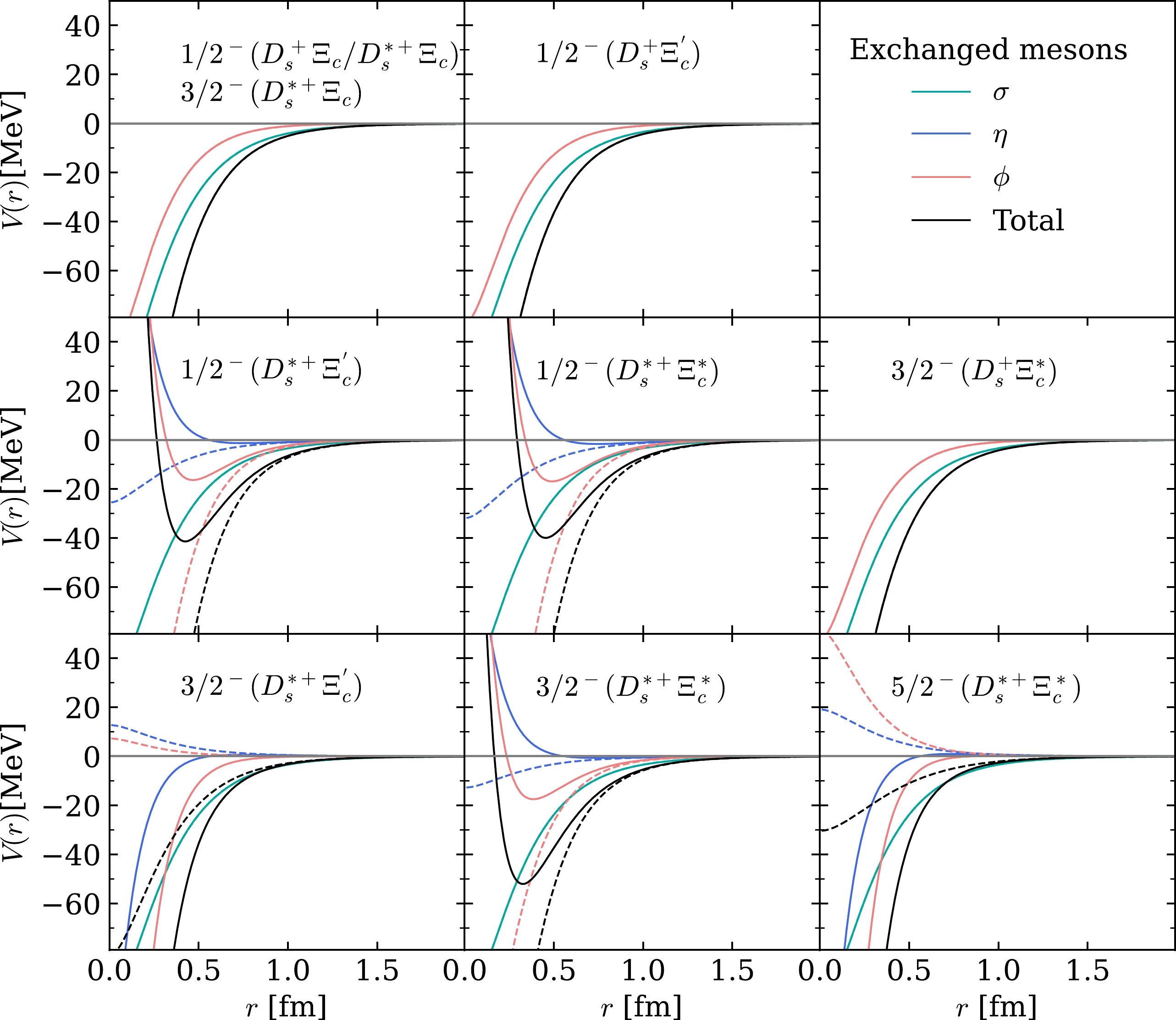oldsymbol{ r }}})$-term.

Figure 1.  (color online) S-wave potentials in single channels with $\Lambda=1.5$ GeV. Solid (dashed) lines correspond to $a=0(1)$, i.e., with (without) the $\delta({{\boldsymbol{ r }}})$-term.

The LHCb $P_c$ pentaquarks were discovered in the analysis of the invariant mass distributions of $J/\psi p$, and their masses are several MeV below the thresholds of $\bar D^{(*)}\Sigma_c$ systems [31, 32]. A natural explanation is that the pentaquarks arise as bound states of $\bar D^{(*)}\Sigma_c^{(*)}$, in which the nonrelativistic potentials for the time-independent Schrödinger equation deduced from the t-channel scattering amplitude are a good description for the interaction of these systems [35−38, 86, 88]. We use the nonrelativistic potentials derived in the previous subsection to explore bound states or resonances in $D^{(*)+}\Xi_c^{('*)}$ systems. For the coupled-channel potential matrix $\mathcal{V}_{jk}$, the radial Schrödinger equation can be written as

where j is the channel index, $u_j$ is defined by $u_j(r)= rR_j(r)$, with the radial wave function $R_j(r)$ for the j-th channel, $\mu_j$ and $W_j$ are the corresponding reduced mass and threshold, respectively, and E is the total energy of the system. The momentum for the channel j is expressed as

By solving Eq. (28), we obtain the wave function, which is normalized to satisfy the incoming boundary condition for the j-th channel [109],

where $S_{jk}(E)$ is the scattering matrix component. In the multi-channel problem, there is a sequence of thresholds, $W_1<W_2<\cdots$, and the scattering matrix element $S_{jk}(E)$ is an analytic function of E, except at the branch points $E=W_j$ and possible poles. Bound/virtual states and resonances are represented as the poles of $S_{jk}(E)$ in the complex energy plane [109].

The characterization of these poles requires analytically extending the S matrix to the complex energy plane, and the poles should be searched for on the correct Riemann sheet (RS). Note that momentum $q_j$ is a double-valued function of energy E, and there are two RSs in the complex energy plane for each channel, one known as the first or physical sheet and the other known as the second or unphysical sheet. In the physical sheet, the complex energy E maps to the upper-half plane (${\rm{Im}}[q_j]\geq 0$) of $q_j$. In the unphysical sheet, the complex energy E maps to the lower-half plane (${\rm{Im}}[q_j]< 0$) of $q_j$. In a coupled-channel system with n channels, the scattering amplitude has $2^n$ RSs, which can be defined by the imaginary part of the momentum $q_j(E)$ of the j-th channel (see Chapter 20 of Ref. [109] for more details). Each RS is labeled by $r=(\pm,\cdots,\pm)$, and the j-th "$\pm$" here denotes the sign of the imaginary parts of the j-th channel momentum $q_j(E)$.

Now, we discuss the possibility of bound {or virtual} states in the $D_s^{+}\Xi_c$, $D_s^{+}\Xi_c^{'}$, $D_s^{*+}\Xi_c$, $D_s^{+}\Xi_c^{*}$, $D_s^{*+}\Xi_c^{'}$, and $D_s^{*+}\Xi_c^{*}$ systems by varying Λ in the range $1.0-2.5$ GeV. Considering the OBE potentials and S-D-wave mixing, the pole positions are obtained by solving the Schrödinger equation in Eq. (28). As discussed in the previous section, the $\delta({{\boldsymbol{ r }}})$-term dominates the short-range dynamics of the potentials and thus serves as the phenomenological contact term, which is used to determine the short-range dynamics of hadron interactions [38]. The proper treatment of $\delta({{\boldsymbol{ r }}})$ in the OBE model plays an important role in the simultaneous interpretation of the LHCb $P_c$ states [88]. Therefore, we represent the results in two extreme cases with $a=0$ or 1.

In the single-channel case, the bound state corresponds to the pole located at the real energy axis below the threshold on the first RS, whereas the virtual state corresponds to the pole at the real energy axis below the threshold on the second RS. The binding energies of the bound or virtual states are defined as

In the single-channel case, the binding energies for these systems with $J^P=1/2^-,3/2^-$, and $5/2^-$ when the cutoff varies from $1.0$ to $2.5$ GeV are shown in Fig. 2. Complementary to this, as shown in Fig. 1, the OBE potentials for the $D_s^{*+}\Xi_c^{'}$ and $D_s^{*+}\Xi_c^{*}$ channels depend on the $\delta({{\boldsymbol{ r }}})$-term, whereas those of the other channels are free of the $\delta({{\boldsymbol{ r }}})$-term. The results for these two channels when the $\delta({{\boldsymbol{ r }}})$-term is removed are given in the three subplots in the right panel of Fig. 2. As shown in the three subplots in the left panel of Fig. 2, ten virtual states are found when $\Lambda=1.0$ GeV, which become bound states as the cutoff increases. In the $J^P=1/2^-$ sector, the $D_s^{+}\Xi_c$, $D_s^{*+}\Xi_c$, and $D_s^{+}\Xi_c^{'}$ states are more easily bound compared to those in the $D_s^{*+}\Xi_c^{'}$ and $D_s^{*+}\Xi_c^{*}$ channels because the $\delta({{\boldsymbol{ r }}})$-terms in the potentials of the latter two channels are repulsive. After removing the $\delta({{\boldsymbol{ r }}})$-term, both the $D_s^{*+}\Xi_c^{'}$ and $D_s^{*+}\Xi_c^{*}$ channels can form relatively deep bound states, as shown in the top-right subplot in Fig. 2. However, the $J^P= 1/2^- D_s^{+}\Xi_c^{*}$ system is in the D-wave and cannot form a bound state. In the $J^P=3/2^-$ sector, the formation of the $D_s^{*+}\Xi_c^{'}$ and $D_s^{*+}\Xi_c^*$ bound states is sensitive to the treatment of the $\delta({{\boldsymbol{ r }}})$-term. For instance, it is more difficult for the $D_s^{*+}\Xi_c^{'}$ system to be bound when the $\delta({{\boldsymbol{ r }}})$-term is removed, whereas the situation is reversed for the $D_s^{*+}\Xi_c^*$ system owing to the opposite sign of the $\delta({{\boldsymbol{ r }}})$-term in these two systems. For the $J^P=5/2^-$ system, only one near-threshold pole is found, corresponding to the $D_s^{*+}\Xi_c^*$ channel. Including the $\delta({{\boldsymbol{ r }}})$-term in this channel makes the binding easier.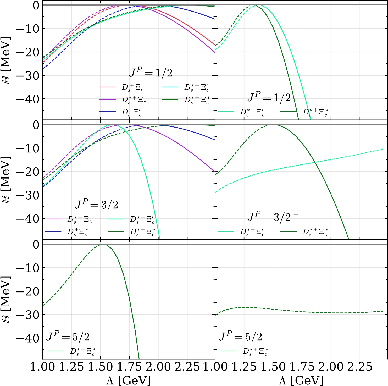

Figure 2.  (color online) Binding energy ($\mathbb{B}$) of the bound states (solid curves) or virtual states (dashed curves) in the single channels as Λ increases. The results without the $\delta({{\boldsymbol{ r }}})$-term are shown in the left panel.

As shown in Ref. [19], when only ϕ meson exchange is considered, the poles in the ten channels mentioned above are located at the second RS below the corresponding thresholds and move toward the thresholds as the cutoff increases in a reasonable range. In this study, we consider the contribution from other meson exchanges, η and σ; hence, the more attractive potentials used in our study together with the $S-D$ wave mixing effect naturally push the poles on the second sheets to the 1st RS when the cutoff is increased. In addition, the formation of the bound states in double charm and hidden strangeness systems, $D_s^{(*)+}\Xi_c^{(',*)}$, is easier than in hidden charm and double strangeness systems, as investigated in Ref. [110].

We further investigate the coupled-channel dynamics of the $D_s^{+}\Xi_c$-$D_s^{+}\Xi_c^{'}$-$D_s^{*+}\Xi_c$-$D_s^{+}\Xi_c^{*}$-$D_s^{*+}\Xi_c^{'}$-$D_s^{*+}\Xi_c^{*}$ system by solving the Schrödinger equation in Eq. (28). Physical resonances are calculated via analytic continuation of the $S(E)$ matrix extracted from the asymptotic wave function in Eq. (30) (see Refs. [109, 111]). In our case of the 6-channel system, there are $2^6$ RSs, labeled as $r= (\pm\pm\pm\pm\pm\pm)$. Note that we only focus on those that are relatively close to the physical real axis. We refer to the review section of Ref. [89] for connections between each RS and the physical real axis.

Because the S-wave component of the coupled channels is important for near-threshold poles and contributions from other higher partial wave components are highly suppressed by centrifugal potentials, we first turn off S-D-wave mixing and only consider the S-wave components to observe the pole trajectories in the $D_s^{+}\Xi_c$-$D_s^{+}\Xi_c^{'}$-$D_s^{*+}\Xi_c$-$D_s^{+}\Xi_c^{*}$-$D_s^{*+}\Xi_c^{'}$-$D_s^{*+}\Xi_c^{*}$ coupled-channel system by varying Λ.

For the $J^P=1/2^-$ system, the five channels $D_s^{+}\Xi_c$-$D_s^{+}\Xi_c^{'}$-$D_s^{*+}\Xi_c$-$D_s^{*+}\Xi_c^{'}$-$D_s^{*+}\Xi_c^{*}$ can couple in the S-wave. In this case, the trajectories of poles near the thresholds of these five channels as the cutoff increases from $1.0$ GeV are shown in Fig. 3, and the similar results after removing the $\delta({{\boldsymbol{ r }}})$-term from the potentials are shown in Fig. 4. When $\Lambda=1.0$ GeV, five near-threshold poles emerge simultaneously on the complex plane, below the thresholds of the five channels; however, they are not directly connected to the physical real axis. They move to the right and approach the thresholds as the cutoff increases. If the cutoff increases up to sufficiently large values such that $1.80,\; 1.70,\; 1.75,\; 2.65$, and $2.40$ GeV are obtained for the five poles below the thresholds of the $D_s^{+}\Xi_c$, $D_s^{+}\Xi_c^{'}$, $D_s^{*+}\Xi_c$, $D_s^{*+}\Xi_c^{'}$, and $D_s^{*+}\Xi_c^{*}$ channels, respectively, these five poles move into other RSs and become directly connected to the physical real axis. As shown in Fig. 4, if the $\delta({{\boldsymbol{ r }}})$-terms are removed from the potential, the poles near the thresholds of $D_s^{*+}\Xi_c^{'}$ and $D_s^{*+}\Xi_c^{*}$ appear in the region connected to the physical real axis with smaller cutoff. Such behavior of these two poles from the effect of the $\delta({{\boldsymbol{ r }}})$-term also mimics that of bound states in the single-channel case of $D_s^{*+}\Xi_c^{'}$ and $D_s^{*+}\Xi_c^{*}$ in the previous subsection.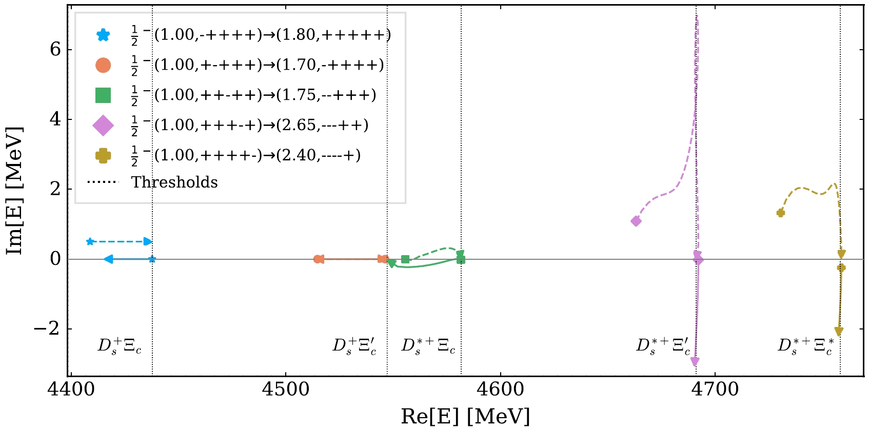

Figure 3.  (color online) Trajectories of the near-threshold poles in the $D_s^{+}\Xi_c$-$D_s^{+}\Xi_c^{'}$-$D_s^{*+}\Xi_c$-$D_s^{*+}\Xi_c^{'}$-$D_s^{*+}\Xi_c^{*}$ channels with $J^P=1/2^-$ by varying the cutoff. For each pole, the dashed (solid) curve represents the trajectory of the pole in the RS, whose label is shown in the left (right) parenthesis in the legend, where the number (in units of GeV) is the starting value of the cutoff. The trajectory of the virtual pole of the $D_s^{+}\Xi_c$ system is artificially moved from the real axis to the complex plane for better illustration.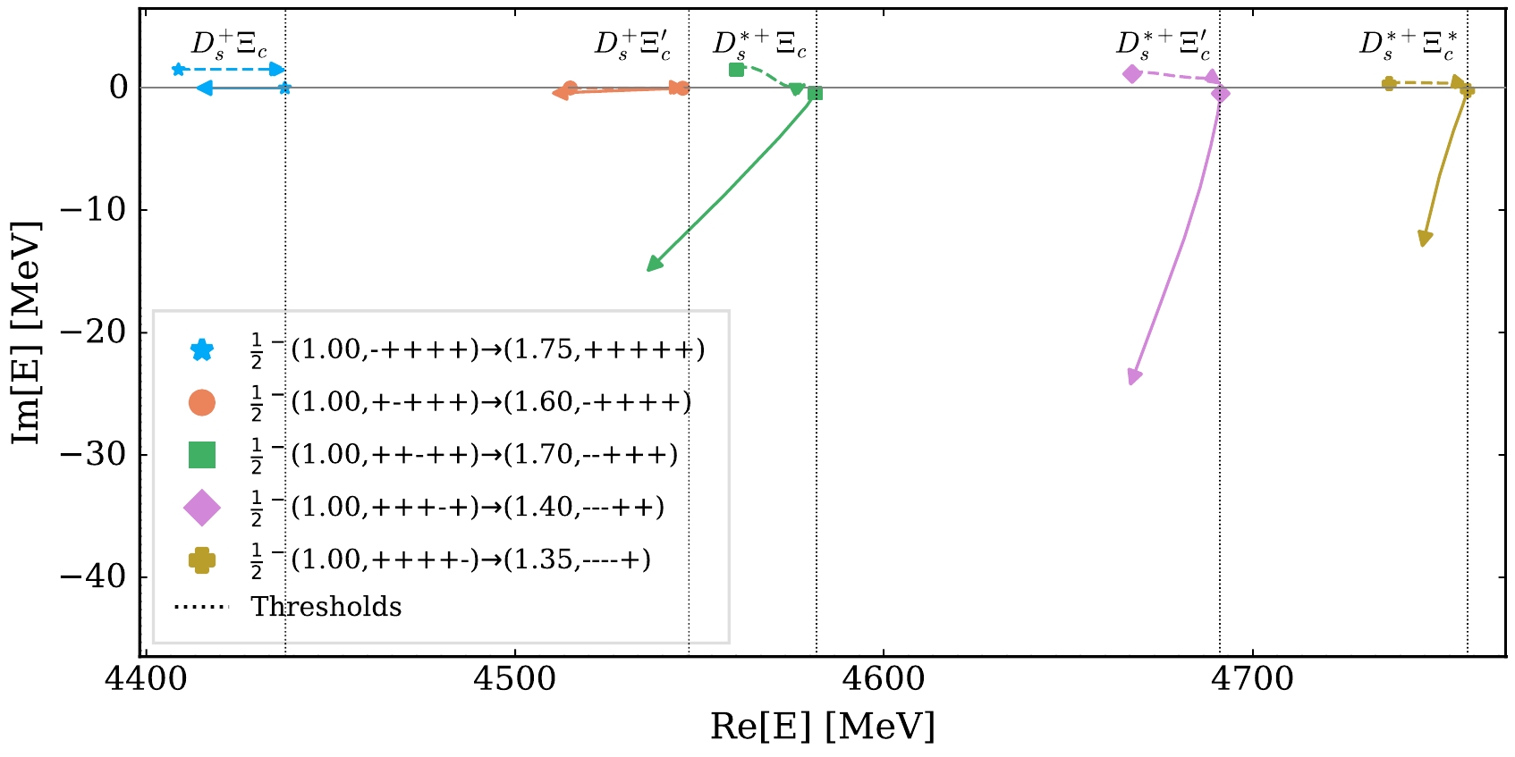

Figure 4.  (color online) Similar to Fig. 3, but after removing the $\delta({{\boldsymbol{ r }}})$-term.

For the $J^P=3/2^-$ system, the four channels $D_s^{*+}\Xi_c$-$D_s^{+}\Xi_c^*$-$D_s^{*+}\Xi_c^{'}$-$D_s^{*+}\Xi_c^{*}$ can couple in the S-wave. The pole trajectories near the thresholds of these four channels as the cutoff increases from $1.0$ GeV are shown in Fig. 5, and the pole trajectories after removing the $\delta({{\boldsymbol{ r }}})$-term are shown in Fig. 6. In both the cases of including and excluding the $\delta({{\boldsymbol{ r }}})$-term, the pole below the threshold of the $D_s^{*+}\Xi_c^{*}$ channel does not appear on the RS connected to the physical real axis within the cutoff range $1.0-3.0$ GeV. ³

Figure 5.  (color online) Trajectory of the near-threshold poles in the $D_s^{*+}\Xi_c$-$D_s^{+}\Xi_c^*$-$D_s^{*+}\Xi_c^{'}$-$D_s^{*+}\Xi_c^{*}$ channels with $J^P=3/2^-$ by varying the cutoff. The trajectory of the virtual pole of the $D_s^{*+}\Xi_c$ system is artificially moved from the real axis to the complex plane for better illustration. See the caption of Fig. 3.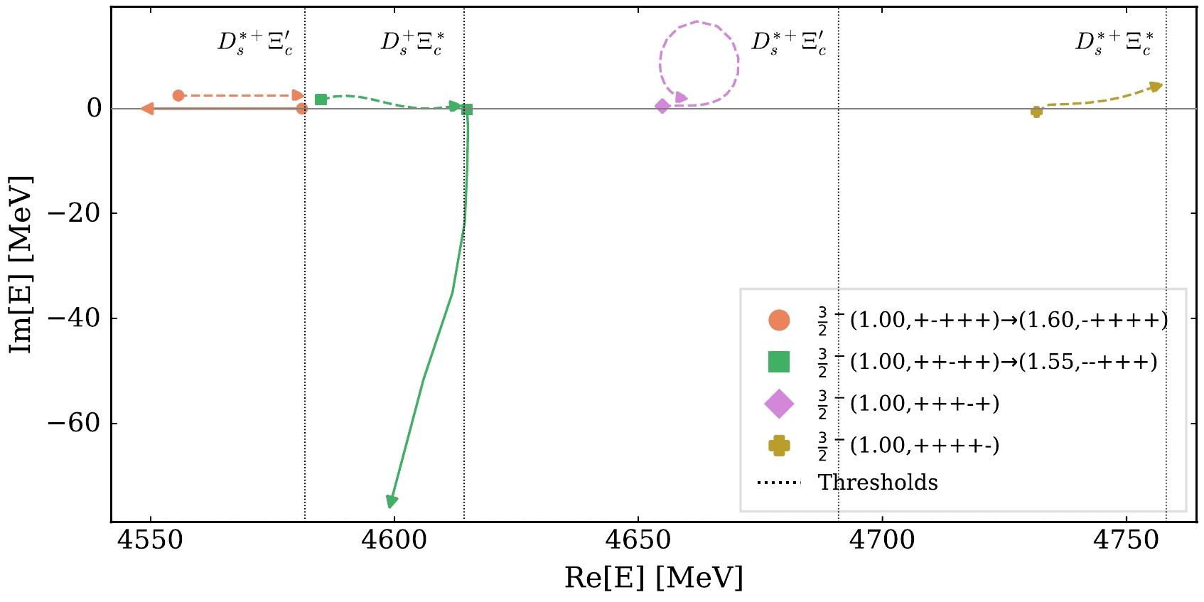

Figure 6.  (color online) Similar to Fig. 5, but after removing the $\delta({{\boldsymbol{ r }}})$-term.

Because only $D_s^{*+}\Xi_c^{*}$ can form the $J^P=5/2^-$ system if only the S-wave is considered, no coupled-channel dynamics appear.

To estimate the contribution of the possible D-wave components, we turn to the S-D-wave mixing potential and calculate the pole positions near the thresholds of the $D_s^{+}\Xi_c$, $D_s^{+}\Xi_c^{'}$, $D_s^{*+}\Xi_c$, $D_s^{+}\Xi_c^{*}$, $D_s^{*+}\Xi_c^{'}$, and $D_s^{*+}\Xi_c^{*}$ channels. The behaviors of these poles by varying the cutoff are presented in Appendix B, which indicates that S-D-wave mixing effects cause the poles to appear on the RS connected to the physical real energy axis with smaller cutoff. In other words, S-D-wave mixing provides additional attractions to these systems. In particular, such effects are more important for poles with $J^P=3/2^-,5/2^-$ near the thresholds of the $D_s^{*+}\Xi_c^{'}$ and $D_s^{*+}\Xi_c^{*}$ channels.

In our calculation, we can determine neither the cutoff Λ nor the reduction parameter a, which represents the contribution of the $\delta({{\boldsymbol{ r }}})$-term, i.e., the short-range interaction, because there is no experimental data on double-charm pentaquarks with hidden strangeness. However, as an illustrative result, we can present full coupled-channel results including S-D-wave mixing effects by fixing the cutoff to $1.5$ GeV, which is somehow phenomenologically reasonable because the LHCb $P_c$ pentaquarks [32] are reproduced with $\Lambda=1.4$ GeV in Ref. [88], with $\Lambda=1.04$ and 1.32 GeV in Ref. [86]. It is mentioned in Ref. [22] that in nucleon-nucleon interactions, values of Λ between 0.8 and 1.5 GeV have been used depending on the model and application, and larger values ($\Lambda > 1.5$ GeV) are also required for nucleon-nucleon phase shifts. By setting $\Lambda=1.5$ GeV, ten poles are found near the thresholds of the $D_s^{+}\Xi_c$, $D_s^{+}\Xi_c^{'}$, $D_s^{*+}\Xi_c$, $D_s^{+}\Xi_c^{*}$, $D_s^{*+}\Xi_c^{'}$, and $D_s^{*+}\Xi_c^{*}$ channels, as shown in Table 2. Among them, the pole below the threshold of the lowest channel $D_s^{+}\Xi_c$ with $J^P=1/2^-$ is a bound state. The poles with imaginary parts, except for those labeled with superscripts "$\bigtriangleup$," are resonances. These poles correspond to the solid lines in Figs. 3 and 5, which are directly connected to the physical real axis and therefore known as "bound-state-like" poles or physical resonances. Conversely, the poles with superscripts "$\bigtriangleup$," corresponding to the dashed lines in Figs. 3 and 5, are not directly connected to the physical real axis and are therefore known as "virtual-state-like" poles. We must emphasize that a "virtual-state-like" pole, although located on the RS remote from the physical real axis, may cause a clear cusp (peak- or dip-like) structure at the threshold if the pole is located close to the threshold. The resonances can decay to lower channels, and the partial decay widths shown in the last column of Table 2 are calculated using the procedure presented in Ref. [104]. Similar results obtained by removing the $\delta({{\boldsymbol{ r }}})$-term from the potentials are shown in Table 3. For the cases without $\delta({{\boldsymbol{ r }}})$, compared to the cases with the $\delta({{\boldsymbol{ r }}})$-term, we find that 1) $1/2^-(D_s^{*+}\Xi_c^{'})$, $1/2^-(D_s^{*+}\Xi_c^{*})$, and $3/2^-(D_s^{*+}\Xi_c^{*})$ become resonances, and 2) $3/2^-(D_s^{+}\Xi_c^{*})$, $3/2^-(D_s^{*+}\Xi_c^{*})$, and $5/2^-(D_s^{*+}\Xi_c^{*})$ turn to "virtual-state-like" poles.

$J^P$	Nearby channel	Threshold/MeV	$E_{\rm pole}$/MeV	$\Gamma_i$($D_s^+\Xi_c/D_s^+\Xi_c'/D_s^{*+}\Xi_c/D_s^+\Xi_c^*/D_s^{*+}\Xi_c/D_s^{*+}\Xi_c^*$)/MeV
$1/2^-$	$D_s^+\Xi_c$	4437.76	$4437.71$	$\cdots$
	$D_s^{+}\Xi_c'$	4547.14	$4547.04-{\rm i}0.01^\bigtriangleup$	$\cdots$
	$D_s^{*+}\Xi_c$	4581.62	$4564.26-{\rm i}1.00$	$0.18/1.81/\cdots/\cdots/\cdots/\cdots$
	$D_s^{*+}\Xi_c'$	4691.00	$4687.07-{\rm i}3.97^\bigtriangleup$	$\cdots$
	$D_s^{*+}\Xi_c^*$	4758.17	$4754.05-{\rm i}4.27^\bigtriangleup$	$\cdots$
$3/2^-$	$D_s^{*+}\Xi_c$	4581.62	$4569.56-{\rm i}0.02$	$0.01/0.04/\cdots/\cdots/\cdots/\cdots$
	$D_s^+\Xi_c^*$	4614.31	$4614.29-{\rm i}0.05$	$0.00/0.02/0.10/\cdots/\cdots/\cdots$
	$D_s^{*+}\Xi_c'$	4691.00	$4689.01-{\rm i}2.58$	$3.36/0.06/1.9/0.36/\cdots/\cdots$
	$D_s^{*+}\Xi_c^*$	4758.17	$4769.34-{\rm i}9.95^\bigtriangleup$	$\cdots$
$5/2^-$	$D_s^{*+}\Xi_c^*$	4758.17	$4727.40-{\rm i}13.37$	$7.82/0.19/19.27/0.33/0.02/\cdots$

Table 2.  Pole positions and partial decay widths of the states in the coupled-channel system of $D_s^{+}\Xi_c$-$D_s^{+}\Xi_c^{'}$-$D_s^{*+}\Xi_c$-$D_s^{+}\Xi_c^{*}$-$D_s^{*+}\Xi_c^{'}$-$D_s^{*+}\Xi_c^{*}$ when $\Lambda=1.5$ GeV with S-D-wave mixing. The poles labeled with the superscript "$\bigtriangleup$" are "virtual-state-like" poles emerging on the RSs far from the physical real axis. Each entry labeled with "$\cdots$" in the column $\Gamma_i$ indicates that the decay is not allowed.

$J^P$	Nearby channel	Threshold/MeV	$E_{\rm pole}$/MeV	$\Gamma_i$($D_s^+\Xi_c/D_s^+\Xi_c'/D_s^{*+}\Xi_c/D_s^+\Xi_c^*/D_s^{*+}\Xi_c/D_s^{*+}\Xi_c^*$)/MeV
$1/2^-$	$D_s^+\Xi_c$	4437.76	$4437.73$	$\cdots$
	$D_s^{+}\Xi_c'$	4547.14	$4547.14-{\rm i}0.00^\bigtriangleup$	$\cdots$
	$D_s^{*+}\Xi_c$	4581.62	$4565.34-{\rm i}2.68$	$0.18/4.98/\cdots/\cdots/\cdots/\cdots$
	$D_s^{*+}\Xi_c'$	4691.00	$4686.30-{\rm i}4.49$	$1.20/6.41/2.02/0.01/\cdots/\cdots$
	$D_s^{*+}\Xi_c^*$	4758.17	$4742.51-{\rm i}6.44$	$2.81/2.57/6.26/0.05/1.46/\cdots$
$3/2^-$	$D_s^{*+}\Xi_c$	4581.62	$4570.09-{\rm i}0.02$	$0.00/0.04/\cdots/\cdots/\cdots/\cdots$
	$D_s^+\Xi_c^*$	4614.31	$4614.26-{\rm i}0.22^\bigtriangleup$	$\cdots$
	$D_s^{*+}\Xi_c'$	4691.00	$4689.71-{\rm i}6.38^\bigtriangleup$	$\cdots$
	$D_s^{*+}\Xi_c^*$	4758.17	$4747.06-{\rm i}16.76$	$2.29/0.02/24.51/7.32/3.89/\cdots$
$5/2^-$	$D_s^{*+}\Xi_c^*$	4758.17	$4763.39-{\rm i}11.20^\bigtriangleup$	$\cdots$

Table 3.  Same as Table 2, but without the $\delta({{\boldsymbol{ r }}})$-term.

From the above results, we find that some states, such as $1/2^-(D_s^{+}\Xi_c^{'})$ and $3/2^-(D_s^{+}\Xi_c^{*})$, are extremely close to their thresholds and will appear as resonances with the additional attraction due to the exchange of $\eta'$ and $f_0(980)$ mesons. Consequently, the pole positions for the other states also move slightly away from the corresponding thresholds owing to this attraction. Up to the masses of the exchanged mesons, the $\eta'$ and $f_0(980)$ exchanges in the $D_s^{(*)+}\Xi_c^{(*,')}$ systems are the same as the η and σ exchanges, respectively, and the potentials of these systems are described in Appendix A. For their coupling constants, we assume that the $f_0(980)$ coupling has the same strength as the σ coupling, and the universal couplings of the pseudoscalar octet mesons $g_1$ and g are adopted for the couplings of $\eta'$ by including it into the ${S U(3)}$ octet of the pseudoscalar meson [112]. The masses of $\eta'$ and $f_0(980)$ are taken as $957.8$ and $990.0$ MeV [89]. With the cutoff $\Lambda=1.5\; \rm{GeV}$, the pole positions for the $1/2^-(D_s^{+}\Xi_c)$, $1/2^-(D_s^{+}\Xi_c^{'})$, $1/2^-(D_s^{*+}\Xi_c)$, $3/2^-(D_s^{*+}\Xi_c)$, $3/2^-(D_s^{+}\Xi_c^{*})$, $3/2^-(D_s^{*+}\Xi_c^{'})$, and $5/2^-(D_s^{*+}\Xi_c^{*})$ states in this case are $4436.81$, $4546.45-{\rm i}0.03$, $4558.57-{\rm i}1.38$, $4564.9-{\rm i}0.11$, $4612.86-{\rm i}0.3$, $4684.02-{\rm i}3.6$, and $4716.58- {\rm i}12.22$ in units of $\rm{MeV}$, respectively. Compared to the results in Table 2, the pole corresponding to the $1/2^-(D_s^{+}\Xi_c^{'})$ state appears at the RS connected to the physical real energy axis, and the other poles are shifted toward the lower thresholds. In the case without the $\delta(r)$-term, the poles labeled with $1/2^-(D_s^{+}\Xi_c^{'})$ and $3/2^-(D_s^{+}\Xi_c^{*})$ appear in the RS connected to the physical real energy axis at the positions of $(4544.84 - {\rm i}0.22)\rm{ \; MeV}$ and $(4613.99 - {\rm i}0.44)\rm{\; MeV}$, respectively. The other poles are also slightly shifted toward the lower threshold.

Note that in the above calculations, $D_s^{+}\Xi_c$ is the lowest channel; therefore, the pole below its threshold is located on the real axis and is stable against the strong interaction. In fact, $D_s^{+}\Xi_c$, as well as other higher channels, can transit into $D^{(*)}\Lambda_c$ or $D^{(*)}\Sigma_c^{(*)}$ via $K^{(*)}$ exchange, which will lead to a finite width of the $D_s^{+}\Xi_c$ bound state. Because we are not aiming at a precise result, we introduce only the $D^{(*)}\Lambda_c$ channels into the previous coupled channels to roughly estimate the decay width of the $1/2^-(D_s^{+}\Xi_c)$ bound state. ⁴ The potentials for the $D^{(*)}\Lambda_c$ channels coupled to the $D_s^{(*)+}\Xi_c^{(*,')}$ channels are listed in Appendix C. The $1/2^-(D_s^{+}\Xi_c)$ bound state now moves into the complex energy plane, and the pole positions along with their partial decay widths are shown in Table 4. We find that the sum of the partial decay widths of the $1/2^-(D_s^{+}\Xi_c)$ bound state to the $D^{(*)}\Lambda_c$ final states is ${\cal O}(1\ \rm MeV)$. For the poles related to other higher channels, we expect similar or larger contributions of the $D^{(*)}\Lambda_c$ channels to their decay widths owing to the larger phase space. Therefore, we consider $D^{(*)}\Lambda_c$ as a good place to search for the predicted states in the $D_s^{+}\Xi_c$-$D_s^{+}\Xi_c^{'}$-$D_s^{*+}\Xi_c$-$D_s^{+}\Xi_c^{*}$-$D_s^{*+}\Xi_c^{'}$-$D_s^{*+}\Xi_c^{*}$ coupled-channel system.

Λ/MeV	$E_{\rm{pole}}$/MeV	$\Gamma_i(D\Lambda_c/D^*\Lambda_c)$/MeV
$1500$	$4437.62-{\rm i}0.37$	$0.88/0.02$
$1600$	$4435.92 -{\rm i}1.12$	$2.04/0.06$

Table 4.  Pole positions and partial decay widths of the $1/2^-(D_s^{+}\Xi_c)$ bound state after including the lower $D^{(*)}\Lambda_c$ channels. The $\delta({{{\boldsymbol{ r }}}})$-term and S-D mixing are considered.

In this study, as partners of $P_c$ pentaquarks, double-charm hidden-strangeness pentaquarks near the $D_s^{+(*)}\Xi_c^{(',*)}$ thresholds are systematically investigated in the hadronic molecular picture. Possible near-threshold states are explored as their molecular candidates within the OBE model. First, the possible bound or virtual states in six single channels, $D_s^{+}\Xi_c$, $D_s^{+}\Xi_c^{'}$, $D_s^{*+}\Xi_c$, $D_s^{+}\Xi_c^{*}$, $D_s^{*+}\Xi_c^{'}$, and $D_s^{*+}\Xi_c^{*}$, are calculated by solving the Schrödinger equation with OBE potentials including S-D-wave mixing. By varying the cutoff in the range $1.0-2.5$ GeV and including the $\delta({{\boldsymbol{ r }}})$-term, five states with $J^P=1/2^-$, four states with $J^P=3/2^-$, and one state with $J^P=5/2^-$ can form virtual states if $\Lambda>1$ GeV, which turn into bound states when Λ becomes sufficiently large. In addition, the results after removing the $\delta({{\boldsymbol{ r }}})$-term are also presented. Second, the coupled-channel dynamics of $D_s^{+}\Xi_c$-$D_s^{+}\Xi_c^{'}$-$D_s^{*+}\Xi_c$-$D_s^{+}\Xi_c^{*}$-$D_s^{*+}\Xi_c^{'}$-$D_s^{*+}\Xi_c^{*}$ are further investigated, and the masses and widths of ten possible resonances and bound states as molecular candidates for double-charm hidden-strangeness pentaquarks are calculated. For the ten molecular states in our coupled-channel analysis, the role of the $\delta({{\boldsymbol{ r }}})$-term in the OBE potentials is also examined. Its influence on the poles near the thresholds of the $D_s^{*+}\Xi_c^{'}$ and $D_s^{*+}\Xi_c^{*}$ channels is most significant. Our study indicates that among these ten poles, the pole with $J^P=1/2^-$ below the$D_s^{+}\Xi_c$ threshold is a bound state, which becomes a resonance after introducing the coupling to the lower $D^{(*)}\Lambda_c$ and $D^{(*)}\Sigma_c^{(*)}$ channels, two poles with $J^P=1/2^-$ and $3/2^-$ below the threshold of the $D_s^{*+}\Xi_c$ channel are physical resonances, and the other seven poles are resonances or "virtual-state-like" poles, depending on the contribution of the $\delta({{\boldsymbol{ r }}})$-term in the OBE model. Further experimental investigations are required to verify these results. These poles may lead to near-threshold structures in the $D^{(*)}\Lambda_c$ final states and can be searched for in the future.

The potentials related to the $D_s^{(*)}\Xi_c^{(',*)}$ channels are shown below.

where $\boldsymbol \epsilon_2$ and $\boldsymbol \epsilon_4^*$ are the polarization vectors for charmed mesons in the initial and final states.

In this section, we show the pole behavior with S-D-wave mixing when varying Λ. In the coupled-channel system with $J^P=1/2^-$, five poles are found as the cutoff varies from $1.45$ to $2.6$ GeV, and their positions are given in Table B1, where the sign of the imaginary part of each channel momentum is shown in the parenthesis. The pole labeled with $E^{\rm I}_{\rm{pole}}$ is located on the real energy axis of RS-I and is a bound state. The poles labeled with $E^{\rm{II}}_{\rm{pole}}$ and $E^{\rm{III}}_{\rm{pole}}$ together with $E^{\rm I}_{\rm{pole}}$ emerge with relatively smaller cutoffs compared to the other two poles labeled with $E^{\rm{VI}}_{\rm{pole}}$ and $E^{\rm{V}}_{\rm{pole}}$. Moreover, the latter two are considerably broader.

Λ	$E_{\rm{pole}}^{\rm{I}}(++++++)$	$E_{\rm{pole}}^{\rm{II}}(-+++++)$	$E_{\rm{pole}}^{\rm{III}}(--++++)$	Λ	$E_{\rm{pole}}^{\rm{V}}(----++)$	$E_{\rm{pole}}^{\rm{VI}}(-----+)$
$1450.0$	$\cdots$	$\cdots$	$4572.86-{\rm i}0.69$	$2450.0$	$4690.37-{\rm i}2.08$	$4736.88-{\rm i}26.43$
$1500.0$	$4437.71$	$\cdots$	$4564.26-{\rm i}1.00$	$2500.0$	$4688.48-{\rm i}4.84$	$4731.39-{\rm i}35.46$
$1550.0$	$4436.76$	$4546.13-{\rm i}0.05$	$4552.59-{\rm i}1.62$	$2550.0$	$4684.87-{\rm i}12.06$	$4726.27-{\rm i}46.64$
$1600.0$	$4434.43$	$4545.90-{\rm i}0.01$	$4536.67-{\rm i}0.27$	$2600.0$	$4675.30-{\rm i}24.38$	$4722.37-{\rm i}59.79$

Table B1.  Pole positions on the RSs close to the physical real axis in the coupled-channel system with $J^P=1/2^-$. Each entry with "$\cdots$" indicates that the pole goes to the other RS far from the physical real axis. Λ and the pole position ($E_{\rm{pole}}^{\rm{RS}}$) are in units of MeV.

With the $\delta({{\boldsymbol{ r }}})$-term in the potentials removed, the positions of the five poles in the $J^P=1/2^-$ system as the cutoff increases are shown in Table B2. In this sector, considerable effects of the $\delta({{\boldsymbol{ r }}})$-term can be observed from the last three poles labeled as $E_{\rm{pole}}^{\rm{III}}$, $E_{\rm{pole}}^{\rm{V}}$, and $E_{\rm{pole}}^{\rm{VI}}$. For instance, after removing the $\delta({{\boldsymbol{ r }}})$-term, the third pole labeled with $E_{\rm{pole}}^{\rm{III}}$ becomes broad, and the fourth and fifth poles labeled with $E_{\rm{pole}}^{\rm{V}}$ and $E_{\rm{pole}}^{\rm{VI}}$ emerge in the region of the RSs connected to the physical real energy axis with relatively smaller cutoffs because these poles are relevant to the bound states in the single channel analysis shown in Fig. 2.

Λ	$E_{\rm{pole}}^{\rm{I}}(++++++)$	$E_{\rm{pole}}^{\rm{II}}(-+++++)$	$E_{\rm{pole}}^{\rm{III}}(--++++)$	$E_{\rm{pole}}^{\rm{V}}(----++)$	$E_{\rm{pole}}^{\rm{VI}}(-----+)$
$1400.0$	$\cdots$	$\cdots$	$4579.28-{\rm i}0.09$	$4690.86-{\rm i}0.79$	$4754.72-{\rm i}2.14$
$1500.0$	$4437.73$	$\cdots$	$4565.34-{\rm i}2.68$	$4686.30-{\rm i}4.49$	$4742.51-{\rm i}6.44$
$1600.0$	$4433.68$	$\cdots$	$4546.50-{\rm i}7.00$	$4676.58-{\rm i}10.59$	$4722.74-{\rm i}12.84$
$1700.0$	$4419.55$	$4545.88-{\rm i}0.01$	$4490.75-{\rm i}0.74$	$4661.41-{\rm i}18.69$	$4697.24-{\rm i}20.24$

Table B2.  Same as Table B1, but the $\delta(\boldsymbol r)$-term is removed.

For the $J^P=3/2$ system, as shown in Table B3, four poles are found as the cutoff increases from $1.4$ to $1.55$ GeV. Three of them, labeled with $E_{\rm{pole}}^{\rm{III}}$, $E_{\rm{pole}}^{\rm{IV}}$, and $E_{\rm{pole}}^{\rm{V}}$, are below the thresholds of the $D_s^{*+}\Xi_c$, $D_s^{+}\Xi_c^{*}$, and $D_s^{*+}\Xi_c^{'}$ channels, whereas the last one, labeled with $E_{\rm{pole}}^{\rm{VI}}$, is above the threshold of the $D_s^{+}\Xi_c^{*}$ channel. After removing the $\delta({{\boldsymbol{ r }}})$-term, the pole $E_{\rm{pole}}^{\rm{III}}$ stays almost the same, and the cutoff dependence of the other poles in this sector changes, as shown in Table B5.

Λ	$E_{\rm{pole}}^{\rm{III}}(--++++)$	$E_{\rm{pole}}^{\rm{IV}} (---+++)$	$E_{\rm{pole}}^{\rm{V}}(----++)$	$E_{\rm{pole}}^{\rm{VI}}(-----+)$
$1400.0$	$4579.95-{\rm i}0.02$	$\cdots$	$\cdots$	$\cdots$
$1450.0$	$4576.07-{\rm i}0.03$	$\cdots$	$4691.46-{\rm i}0.79$	$4767.11-{\rm i}2.60$
$1500.0$	$4569.56-{\rm i}0.02$	$4614.29-{\rm i}0.05$	$4689.01-{\rm i}2.58$	$4769.34-{\rm i}9.95$
$1550.0$	$4560.07-{\rm i}0.01$	$4612.57-{\rm i}0.28$	$4683.28-{\rm i}4.09$	$4771.33-{\rm i}20.23$

Table B3.  Same as Table B1, but with $J^P=3/2^-$.

For the $J^P=5/2^-$ system, only one pole is found. The positions of the pole considering the coupled-channel potential with or without the $\delta({{\boldsymbol{ r }}})$-term are shown in Table B4. Compared to the poles near the thresholds of the $D_s^{*+}\Xi_c'$ and $D_s^{*+}\Xi_c^*$ channels in coupled-channel systems with $J^P=1/2^-$ and $3/2^-$, the effect of the $\delta({{\boldsymbol{ r }}})$-term on the pole in the $J^P=5/2^-$ sector is not significant. Among these ten poles, the $E_{\rm{pole}}^{\rm{I,II,III}}$ poles in the $J^P=1/2^-$ system, $E_{\rm{pole}}^{\rm{III,IV}}$ poles in the $J^P=3/2^-$ system, and $E_{\rm{pole}}^{\rm{VI}}$ pole in the $J^P=5/2^-$ system are not sensitive to the $\delta({{\boldsymbol{ r }}})$-term and can appear with relativity smaller cutoffs, whereas the other poles near the thresholds of the $D_s^{*+}\Xi_c'$ and $D_s^{*+}\Xi_c^*$ channels in the $J^P=1/2^-,3/2^-$ systems have different behaviors in the cases with and without the $\delta({{\boldsymbol{ r }}})$-term. In each case, the poles near the thresholds of the $D_s^{*+}\Xi_c'$ and $D_s^{*+}\Xi_c^*$ channels are broad and difficult to observe.

Λ	$E_{\rm{pole}}^{\rm{III}} (--++++)$	$E_{\rm{pole}}^{\rm{IV}}(---+++)$	$E_{\rm{pole}}^{\rm{V}}(----++)$	$E_{\rm{pole}}^{\rm{VI}} (-----+)$
$1500.0$	$4570.09-{\rm i}0.02$	$\cdots$	$\cdots$	$4747.06-{\rm i}16.76$
$1600.0$	$4543.47-{\rm i}0.03$	$4613.45-{\rm i}1.14$	$\cdots$	$4723.38-{\rm i}25.74$
$1700.0$	$4511.62-{\rm i}0.00$	$4606.96-{\rm i}3.86$	$\cdots$	$4693.00-{\rm i}27.76$
$1780.0$	$4509.34-{\rm i}0.00$	$4594.41-{\rm i}5.62$	$4697.89-{\rm i}1.80$	$4666.32-{\rm i}23.34$

Table B4.  Same as Table B3, but the $\delta(\boldsymbol r)$-term is removed.

With $\delta(\boldsymbol r)$			Without $\delta(\boldsymbol r)$
Λ	$E_{\rm{pole}}^{\rm{VI}}(-----+)$		Λ	$E_{\rm{pole}}^{\rm{VI}}(-----+)$
$1350.0$	$4759.44-{\rm i}4.93$		$1400.0$	$4767.33-{\rm i}0.00$
$1400.0$	$4753.08-{\rm i}9.21$		$1500.0$	$4763.39-{\rm i}11.20$
$1450.0$	$4742.35-{\rm i}12.21$		$1600.0$	$4745.55-{\rm i}21.61$
$1500.0$	$4727.40-{\rm i}13.37$		$1700.0$	$4717.43-{\rm i}23.05$

Table B5.  Position of a pole in the coupled-channel system with $J^P=5/2^-$. Λ and the pole position ($E_{\rm{pole}}^{\rm{RS}}$) are in units of MeV.

With the procedure described in Sec. IIB, the effective potentials in the momentum space for the $D^{(*)}\Lambda_c$ channels coupled to the $D_s^{(*)+}\Xi_c^{(',*)}$ channels are derived using the Lagrangian in Eq. (2) and shown below.

where the masses of the relevant particles are $m_\omega=782.7$ MeV, $m_K=493.7$ MeV, and $m_{K^*}=891.7$ MeV.