


 Abstract
 HTML
HTML Reference
 Related
 PDF
PDF


-
In 2012, the ATLAS and CMS collaboration announced the discovery of the Higgs Boson at the Large Hadron Collider (LHC) [1, 2]. In the following years, precise measurements of Higgs properties became one of the main goals in particle physics, aiming to answer the remaining basic questions in nature and find new physics. For this purpose, hadron colliders such as the LHC may not be the best choice owing to the large amount of background processes and corresponding lower ratio between the signals and backgrounds. Instead, a lepton collider can provide a cleaner experiment environment and well-known initial states, which is crucial for high precision studies to find hints of new physics. Thus, several future lepton collider experiments have been proposed, including the International Linear Collider (ILC) [3], Circular Electron Positron Collider (CEPC) [4], Future Circular Collider
e+e− (FCC-ee) [5], and Compact Linear Collider (CLIC) [6].The CEPC was designed to be a circular lepton collider hosted in a tunnel with a circumference of 100 km and operate at a center of mass energy
√s=240 GeV as a Higgs factory. After a 10 year running period, the CEPC will collect 5.6 ab–1 data, corresponding to more than one million Higgs bosons. With this clean and large Higgs sample, the precision of the measurements of Higgs properties is expected to be enhanced by one order of magnitude with respect to the LHC precision [7].The Higgs boson interacts with a photon through the top quark and massive boson loops. This mechanism implies a low
H→γγ branching ratio in the Standard Model (SM) but also makes it a good channel to test new physics beyond the SM. Besides, high energy photons from the Higgs boson decay can be identified and measured well experimentally. Thus, this channel also serves as a good benchmark for the performance of the electromagnetic calorimeter (ECAL) study. Current measurements of the inclusive Higgs boson signal strength in the diphoton channel in the LHC are1.04+0.10−0.09 in ATLAS [8] and1.03+0.11−0.09 in CMS [9], according to thepp collision data collected by ATLAS and CMS from 2015 to 2018. These results are consistent with the SM prediction and present precision. In the HL-LHC period, the ATLAS is expected to collect 3 ab–1 data. The projected precision of theH→γγ measurements ranges from 6% to 4% depending on different considerations concerning systematic uncertainties S1 or S2 reported in [10]. Combined with CMS, a precision of 2.5% can be reached in the optimistic systematic scenario S2.A previous analysis studied the expected Higgs precision in various Higgs decay channels [7] including
H→γγ . A precision of 6.8% is expected for the measurement ofσ(ZH)×Br(H→γγ) with the CEPC-v4 conceptual detector. However, this result is based on fast simulation of Monte Carlo samples and cut-based analysis method. In a recent study [11], the CEPC accelerator study group updated the radiation power, resulting in an increase of the instantaneous luminosity of 66%. Based on this update, a new nominal data-taking scenario was proposed. It aims at ten years of data collected at√s = 240 GeV with two interaction points (IPs), accumulating an integrated luminosity of 20 ab–1 Higgs data [12]. Moreover, a new conceptual detector design is also ongoing. A homogeneous ECAL is considered to replace the previous silicon-tungsten sampling calorimeter [12–14]. Thus, it is worth revisiting theH→γγ process with the latest benchmark and investigating the impact from larger statistics and the new detector.This paper is organized as follows. Section II briefly introduces the CEPC detector and simulated Monte-Carlo samples used in this analysis. Section III presents the object reconstructions and event selections. Section IV describes the MVA method developed in this study. Section V analyzes the signal and background models. The results are summarized in Sec. VI. In Sec. VII, we investigate how these results can be influenced by the CEPC ECAL resolution, which can provide guidelines for detector optimization. The conclusions are drawn in Sec. IX.
-
The CEPC detector was designed to accomplish the physics goal that all final states can be identified and reconstructed with high resolution. The baseline detector concept is based on the particle flow approach (PFA) idea [15]. It comprises a precise vertex detector, a Time Projection Chamber (TPC), a silicon tracker, a high granularity Silicon-Tungsten sampling ECAL, and a GRPC-based high granularity hadronic calorimeter (HCAL). The whole system is embedded in a 3 Tesla magnetic field. The outermost part of the detector is a muon chamber. Further details can be found in Ref. [4].
The Higgs production mechanisms at the CEPC are Higgs-strahlung
e+e−→ZH ,W/Z fusione+e−→νˉνH , ande+e−→e+e−H , as illustrated in Fig. 1. In this analysis, Higgs production via ZH process decaying to diphoton final statee+e−→ZH→fˉfγγ at√s=240 GeV is considered the dominant signal. It is further divided into three sub-channels, depending on Z decaying toqˉq ,μ+μ− , andνˉν . TheZ→e+e− channel is dismissed owing to the well-known extremely large Bhabha background. Likewise, theZ→τ+τ− channel is dismissed because of the complexity of τ identification. TheW/Z fusion process is considered in the ZH,Z→νˉν sub-channel. The only considered background process is the 2-fermion backgrounde+e−→fˉf in CEPC with at least two photons from the initial and final state radiations. The Higgs resonant background, 4-fermion processes, and possible reducible background in the experiments are expected to be negligible. These SM physical processes are generated with Whizard [16] at leading order (LO) interfaced with Pythia 6 [17] for parton showering and hadronization, and parameters based on Large Electron Positron Collider (LEP) [18] data. Initial state radiation (ISR) and final state radiation (FSR) effects are taken into account. The total energy spread caused by beamstrahlung and synchrotron radiation was studied through Monte-Carlo simulation and determined to be 0.1629% at CEPC [19]. Table 1 lists the cross sections of physical processes and MC sample statistics used in the analysis. Event yields were normalized to 5.6 ab–1. Details on the configurations can be found in Ref. [20].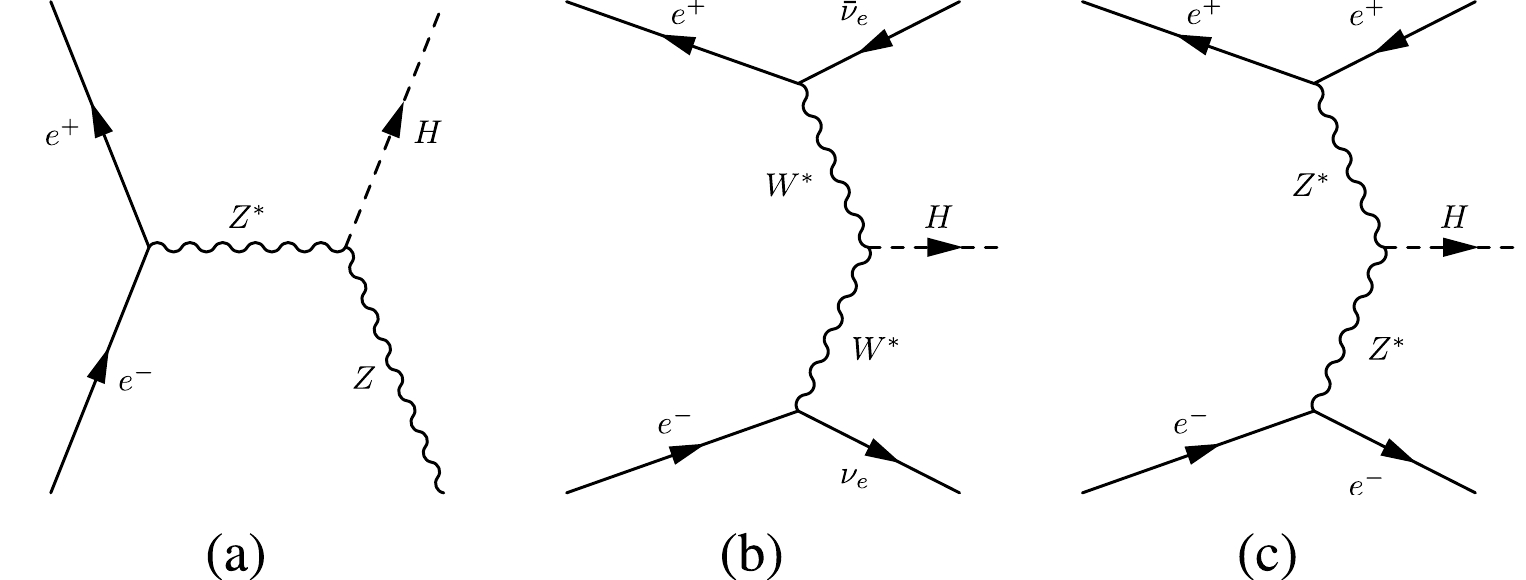
Figure 1. Feynman diagrams of the Higgs boson production processes at the CEPC: (a)
e+e−→ZH , (b)e+e−→νˉνH , and (c)e+e−→e+e−H .Process σ statistics qˉqγγ sub-channel

e+e−→ZH→qˉqγγ 

0.31 fb 100 k e+e−→qˉq 

54.1 pb 20 M μ+μ−γγ sub-channel

e+e−→ZH→μ+μ−γγ 

0.15 fb 100 k e+e−→μ+μ− 

5.3 pb 20 M νˉνγγ sub-channel

e+e−→ZH→νˉνγγe+e−→νˉνH→νˉνγγ 

0.11 fb 100 k e+e−→νˉν 

54.1 pb 20 M Table 1. Cross sections and simulated MC sample statistics. In the
qˉqγγ andμ+μ−γγ channels,ZH is the only process considered, and in theνˉνγγ channel, both ZHZ→inv. andW/Z fusion processes are considered.The simulations of the detector configuration and response were conducted with MokkaPlus [21], a GEANT4 [22] based framework. The full detector simulation was performed for signal processing only. The background processes were simulated by smearing the truth particles with the parameterized detector resolution and efficiency to save computing resources.
-
The CEPC follows the PFA scheme for event reconstruction, with a dedicated tookit ARBOR [23, 24]. The tracks are first reconstructed with the hits in the tracking detector by the Clupatra module [25]. Then, ARBOR collects the tracks from Clupatra and hits in the calorimeter, and composes the Particle Flow Objects (PFOs) using clustering and matching modules. These PFOs are identified as charged particles, photons, neutral hadrons, and unassociated fragments. With this approach, a photon is identified in ARBOR with the shower shape variables obtained from the high granularity calorimeter, without any matched tracks. Converted photons are not considered yet; they amount to 5%–10% in the central region and 25% in the forward region [4]. The lepton (
e±,μ± ) is defined by a track-matched particle. A likelihood-based algorithm, namely LICH [26], is implemented in ARBOR to separate electrons, muons, and hadrons. Jets are formed from the particles reconstructed by ARBOR with the Durham clustering algorithm [27] after excluding the particles of interest. The jet energy is currently calibrated using MC simulation, but it is foreseen to be re-calibrated with physical events such asW→qˉq and/orZ→qˉq in CEPC. No flavor tagging approach was used in this analysis for simplicity.The event selections are applied to improve the signal significance and background modeling. Individual strategies are considered in the three sub-channels depending on the topology of the physical process. In the
ZH→νˉνγγ channel, two photons are required inclusively in the final state. In theZH→μ+μ−γγ channel, the two leading photons and two muons are exclusively selected, requiring a veto of other particles, with the missing energyEmissing and missing massMmissing less than 10 GeV and the invariant mass of the muon pair close to the Z boson mass.In the
ZH→qˉqγγ channel, two leading photons are first selected, and other particles are reconstructed into two jets using the Durham algorithm. Some dedicated cuts are applied on the kinematic variables of these final state objects as listed in Tables 2, 3, 4, along with the final efficiency and expected event yields.Selections Higgs signal qˉqγγ background

Exclusive 2 jets and 2 photons 85.56% 69.57% Eγ1> 25 GeV

100.00% 2.35 % Eγ2∈[35,95] GeV

98.37% 35.33% cosθγγ> –0.95

95.20% 68.01% cosθjj> –0.95

90.86% 85.54% pTγ1> 20 GeV

93.42% 56.94% pTγ2> 30 GeV

93.25% 54.54% mγγ∈[110,140] GeV

97.50% 21.14% Eγγ> 120 GeV

99.47% 98.41% min|cosθγj|<0.9 

71.67% 48.05% Total eff 44.08% 0.01% Yields in 5.6 ab−1 766.64 26849.38 Table 2. Selection criteria and corresponding efficiencies in the
qˉqγγ channel.γ1(γ2) is defined as the photon with lower (higher) energy,cosθγγ(cosθjj) is the polar angle of the di-photon (di-jet) system, andmin|cosθγj| is the minimumcosθ of the photon-jet pairs.Selections Higgs signal μ+μ−γγ background

Exclusive 2 muons and 2 photons 70.18% 5.18% Eγ>35 GeV

99.21% 8.39% |cosθγ|< 0.9

83.79% 38.14% pTγ1∈[10,70] GeV

99.84% 86.30% pTγ2∈[30,100] GeV

99.96% 95.59% mγγ∈[110,140] GeV

98.08% 37.62% Mrecoil γγ∈[85,105] GeV

80.12% 21.29% Eγγ∈[125,145] GeV

99.88% 95.86% Total eff 45.69% 0.01% Yields in 5.6 ab−1 39.32 2662.77 Table 3. Selection criteria and corresponding efficiencies in the
μ+μ−γγ channel.γ1(γ2) is defined as the photon with lower (higher) energy;Mrecoilγγ is the recoil mass of the di-photon system in CEPC√s=240GeV:(Mrecoil γγ)2=(√s−Eγγ)2−p2γγ= s−2Eγγ√s+m2γγ .Selections Higgs signal νˉνγγ background

Inclusive 2 photons 85.51% 0.34% Eγγ> 30 GeV

99.81% 20.13% |cosθγ|< 0.8

70.48% 11.56% pTγ> GeV

99.97% 99.26% Mmissing> 60 GeV

98.17% 99.71% mγγ∈[110,140] GeV

97.51% 22.86% Eγγ∈[120,150] GeV

99.16% 99.58% Total eff 57.08% 0.002% Yields in 5.6 ab−1 335.89 3640.20 Table 4. Selection criteria and corresponding efficiencies in the
νˉνγγ channel.Mmissing is the missing mass calculated from the total visible objects. -
The Multi-Variate Analysis (MVA) method is employed to further suppress the background. It exploits machine learning (ML) techniques to combine the separation power from several variables into a unique variable. In this study, we chose the Gradient Boosted Decision Tree (BDTG) method and TMVA toolkit [28]. For each sub-channel, the ZH and two fermion processes were considered as the signal and background for the BDTG. All events from MC were separated into two sets for 2-fold validation [29] to avoid the risk of overtraining. The following principles were considered while constructing the input variables for BDTG:
● The basic information is the Lorentz vector of the final state particles. This includes the momentum (P), transverse momentum (pT), energy (E), polar angle (
cosθ ), and recoil mass for photons, fermions, and systems;ΔP,ΔE,ΔΦ,Δcosθ,ΔR for two objects or systems; and the missing massMmissing .● The separation
⟨S2⟩ defined in Eq. (1) is used to quantify the discrimination power between signal and background of a given variable, where y represents the discriminating variable, andˆys(y) andˆyb(y) are the corresponding probability distribution function of the variable for signal and background samples, respectively.⟨S2⟩=12∫(ˆys(y)−ˆyb(y))2ˆys(y)+ˆyb(y)dy.

(1) ● To ensure the application of the 2D model described in Sec. V, which requires an assumption of independence between the BDTG response and
mγγ , the constructed variable should have a low linear correlation withmγγ :|Corrv−mγγ|<30% .● To reduce the training redundance, the linear correlation between any two variables should be small:
|Corrv1−v2|<40% . The one with lower separation power is removed.Tables 5–7 lists the selected variables along with their definition and
⟨S2⟩ for BDTG. Their distributions can be found in Appendix A (Figs. A1, A3, A5). The ROC curves and distributions of the trained BDTG are also shown in Appendix A (Figs. A2, A4, A6).Variable Definition Separation pTγ1 

Transverse momentum of the sub-leading photon 0.209 cosθγ2 

Polar angle of the leading photon 0.197 ΔΦγγ 

Azimuthal angle between two photons 0.147 minΔRγ,j 

Minimum ΔR between one of the two photons and one of the jets

0.054 Ej1 

Energy of the sub-leading jet 0.041 ΔΦγγ,jj 

Azimuthal angle between the diphoton and dijet system 0.033 pTj2 

Transverse momentum of the leading jet 0.032 cosθj1 

Polar angle of the sub-leading jet 0.032 cosθγγ,jj 

Polar angle difference between diphoton and dijet system, cos(θγγ−θjj) 

0.024 cosθγ1,j1 

Polar angle difference between sub-leading photon and sub-leading jet, cos(θγ1−θj1) 

0.023 Table 5. Input variables for BDTG in the
qˉqγγ channel.Variable Definition Separation minΔRγ,μ 

Minimum ΔR between one of the two photons and one of the muons

0.335 Eμμ 

Energy of the di-muon system 0.259 cosθγ1,μ1 

Polar angle difference between the sub-leading photon and sub-leading muon 0.189 Eγ2 

Leading photon energy 0.160 ΔΦγγ 

Azimuthal angle between two photons 0.090 cosθγ2 

Polar angle of the leading photon 0.072 ΔΦγγ,μμ 

Azimuthal angle between the diphoton and dimuon system 0.034 cosθμ1 

Polar angle of the sub-leading muon 0.014 Table 6. Input variables for BDTG in the
μ+μ−γγ channel.Variable Definition Separation pTγ1 

Transverse momentum of the sub-leading photon 0.089 cosθγ2 

Polar angle of the leading photon 0.079 ΔΦγγ 

Azimuthal angle between two photons 0.054 pTtγγ 

Diphoton pT projected perpendicular to the diphoton thrust axis 0.042 pTγ2 

Transverse momentum of the leading photon 0.037 Table 7. Input variables for BDTG in the
νˉνγγ channel. -
The Higgs signal is extracted by fitting
mγγ and the shape of the BDTG responses. The resonant peak above a smoothmγγ distribution for the background at around the Higgs mass (125 GeV) can be reconstructed through the excellent calorimeter energy resolution in CEPC. The signalmγγ distribution is fitted with a Double Side Crystal Ball (DSCB) function:f(t)=N×{e−t2/2,if −αlow≤t≤αhighe−12α2low[1Rlow(Rlow−αlow−t)]nlow,if t<−αlowe−12α2high[1Rhigh(Rhigh−αhigh+t)]nhigh,if t>αhigh

(2) where N is a normalization factor and
t=(mγγ−μCB)/σCB . Figure 2 shows the fittedmγγ signal shape in three channels. They are well described by the DSCB function. The resolution is estimated to be 2.81 / 2.68 / 2.74 GeV in theqˉqγγ/μ+μ−γγ/νˉνγγ channels, respectively.
Figure 2. (color online) Signal MC and fitted DSCB model in the three channels.
Several smooth functions (Cheybyshev polynomials, and exponential and polynomial families) were tested for background modeling, and the one with the smallest
χ2 /Ndof value was finally selected. The results are listed in Table 8 and shown in Fig. 3. Details on the fitting conditions for all functions are provided in Appendix A (Table A1 and Fig. A7).Channel Selected function χ2 /Ndof

qˉqγγ 

2nd order Chebyshev 0.60 μ+μ−γγ 

2nd order Chebyshev 1.79 νˉνγγ 

1st order Chebyshev 3.32 Table 8. Decided background model in the three channels. Tested functions include the exponential, 2nd order exponential polynomial, 1st and 2nd order polynomials, and 1st and 2nd order Chebyshev polynomials.
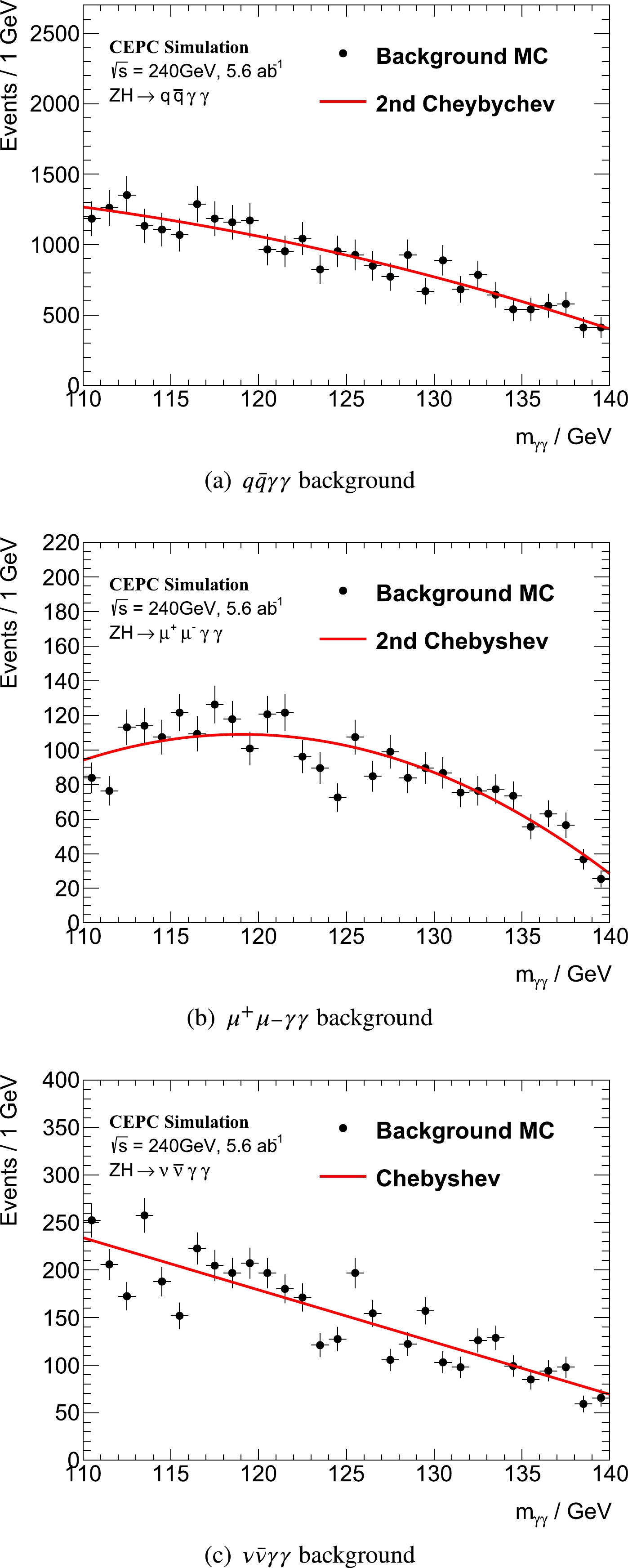
Figure 3. (color online) Background MC and fitted
mγγ models in the three channels.The histograms from the MC of signal and background were used to build the binned Probability Density Function (PDF), which was in turn used as the model of BDTG distributions.
The strategies employed for constructing BDTG ensured the reasonable independence between the BDTG response and
mγγ . Therefore, a 2-dimensional model resulting from the multiplication ofmγγ and BDT models was applied to describe the signal and background. A high correlation can introduce improper modeling of the signal and/or background process. The linear correlation coefficients betweenmγγ and BDT are −3.45%, −11.6%, 8.33% for the signals in theqˉqγγ ,μ+μ−γγ , andνˉνγγ channels, respectively. The corresponding correlation coefficients for the background are 11.6%, 28.2%, and 28.4%, respectively. -
The systematic uncertainties relevant to the targeted measurement can be caused by several sources. However, at this stage, most of them have not been specifically studied yet for the CEPC. Therefore, in this paper, we only present a methodology for analyzing the systematic CEPC uncertainties and taking the leading terms into account. Further quantified analysis requires updates on theoretical calculations, a more comprehensive detector performance optimization, and real data.
Based on the strategy of event modeling presented in Sec. V, the systematic uncertainties can be categorized into two types: uncertainties in the expected signal yields in each channel and uncertainties in the modeling of the signal
mγγ distribution. The background yields andmγγ model parameters are floated to consider the effect of improper background modeling and contributions from model-dependent background process cross section calculations. The uncertainty of BDT modeling for both signal and background is contained by an envelope, which is included into the signal event yield uncertainty.These systematic terms are incorporated into the likelihood model as nuisance parameters. For each of such nuisance parameters, a Gaussian or log-normal constraint PDF is included in the likelihood function, as well as for symmetric terms such as the
mγγ shape peak position or non-negative terms such as the event yield. The construction of likelihood with these nuisance parameters is presented in Sec. VII. -
In contrast to hadron colliders, only few theoretical uncertainties can affect the measurements in lepton collision experiments such as CEPC. The theoretical calculations are less dependent on higher order QCD radiative correction. Moreover, there is no influence from the Parton Distribution Functions or
αS . In thisσ×Br measurement, the observed event yields are directly obtained from fitting, so the uncertainties from signal cross section calculation andBr(H→γγ) can be eliminated. The only remaining uncertainty is the parton shower uncertainty in theqˉqγγ channel. It can be described by the MC sample difference from a set of generators, which is assumed to be negligible. For completeness, a 0.5% theoretical uncertainty is assumed on the signal yield in theqˉqγγ channel. -
The experimental systematic uncertainties affecting this measurement can include integrated luminosity, detector acceptance, trigger efficiency, object reconstruction and identification efficiency, and object energy scale and resolution. In CEPC, the luminosity can be monitored by the Lumi-Cal with the highly statistical BhaBha process. Thus, a relative accuracy of 0.1% is expected [4]. Pile-up effects and underlying events should be negligible. A well-described detector geometry in the simulation is able to provide a precise model of the detector acceptance and response. Possible modeling deviation can be fixed with some data-driven methods. As a result, the uncertainties should be very small. The photon reconstruction, identification, and energy calibration rely on dedicated algorithms and real data. In CEPC CDR, these uncertainties are studied to be controlled with sub-percent level. Furthermore, known physical processes can be used as standard candles for calibration, e.g.,
Z→e+e−+γ andπ0→γγ . Similarly, electrons, muons, and jets can be described well, in principle. In this di-photon channel study, the photon related uncertainties should be dominant. Thus, we assume a 1% uncertainty on the photon efficiency and 0.05% uncertainties on the photon energy scale (PES) and resolution (PER). Other terms remain to be added with better understanding about the experiments.The signal yield is affected by the luminosity, photon efficiency, and impact of the photon energy scale and resolution uncertainties on the selection efficiency. A set of alternative simulation samples are generated, randomly rejecting 1% photons, scaling the energy up/down by 0.05%, or smearing the photon energy with 0.05%. The expected signal yields are counted after all the selections, and a relative variation
δni=|nivar−ninom|ninom is used to represent the influence from each term. This photon efficiency is approximately 2%, and the photon energy scale and resolution are approximately 0.01%. They are considered as symmetric uncertainties on the signal yield.The signal
mγγ distribution is described with the double-side crystal ball function. The photon energy scale uncertainty is propagated to the peak position of the signal peak, whereas the photon energy resolution uncertainty is propagated to the signal width. They are estimated by refitting the signal shape in the variation samples and comparing with the nominal one:δμCB= μCB,var−μCB,nomμCB,nom ,δσCB=σCB,var−σCB,nomσCB,nom . The impact from PES to the signal peak ranges from 0.04% to 0.10% for the different channels, and the impact from PER to the signal width ranges from 0.004% to 0.02%. A 5.9 MeV Higgs mass measurement uncertainty is also considered based on CEPC estimation [7].The influence from these aforementioned uncertainties on BDT modeling is studied by comparing the BDT distribution bin by bin between the nominal and variation MC samples. The maximum variation value
δn=|nvar−nnom|nnom in all BDT bins and systematic terms is applied on the signal yield as the uncertainty from BDT, except for the bin with low statistics (bin content less than 5% of total yield). The uncertainty from BDT itself is assumed to be included in this envelope value. This term ranges from 0.5% to 0.7% for the three channels. -
The number of expected signal events was extracted by combining the fitting in the three channels with the unbinned maximum likelihood fitting method. The likelihood function was built using the models presented in Sec. V and the constraints derived from the systematic uncertainties presented in Sec. VI:
\begin{aligned}[b] \mathcal{L}(\mu,{\boldsymbol{\theta}};({m_{\gamma \gamma }}, \text{BDT})) & = \prod_{c}\text{Pois}(n_c|N_c(\mu, {\boldsymbol{\theta}}))\cdot \\ & \prod_{i}^{n}f_{c}(({m_{\gamma \gamma }}, \text{BDT})^{i};{\boldsymbol{\theta}}) \cdot \prod_{j} G(\theta_j), \end{aligned}

(3) where
● μ is the signal strength expressed as
\mu = \dfrac{N\ (e^{+} e^{-} \to ZH \to f\bar {f}\gamma \gamma)} {N_{\rm SM}\ (e^{+} e^{-} \to ZH \to f\bar {f}\gamma \gamma)} , which is the parameter of interest (POI) in the fitting;●
{\boldsymbol{\theta}} denotes nuisance parameters defined for systematic terms;●
n_c is the observed event number in the channel c from the data;●
N_c(\mu, {\boldsymbol{\theta}})=\mu S_{{\rm SM}, c}({\boldsymbol{\theta_{\rm yield}}}) + B_c .S_{{\rm SM}, c}({\boldsymbol{\theta_{\rm yield}}}) is the expected signal yield in the channel, including the relevant nuisance parameters.B_c is the background yield;●
f_{c}(({m_{\gamma \gamma }}, \text{BDT})^{i};{\boldsymbol{\theta}}) is the probability density function built with the signal and background models presented in Sec. V:\begin{aligned}[b] f_{c}(({m_{\gamma \gamma }}, \text{BDT})^{i};{\boldsymbol{\theta}}) =& \frac{1}{N_c}\times \Big[ \mu S_{{\rm SM}, c}({\boldsymbol{\theta_{\rm yield}}})f_{c,\rm sig}(({m_{\gamma \gamma }},\text{BDT})^i;{\boldsymbol{\theta}}) \\&+ B_{c} f_{c,\rm bkg}(({m_{\gamma \gamma }},\text{BDT})^i;{\boldsymbol{\theta}}) \Big]. \end{aligned}

(4) ● The signal yield
S_{{\rm SM},c} , shape peak\mu_{\rm CB} , and width\sigma_{\rm CB} are affected by systematic uncertainties with a response function:\begin{aligned}[b] S_{{\rm SM},c}({\boldsymbol{\theta_{\rm yield}}})=S_{{\rm SM},c}\prod\limits_{j}{\rm e}^{\theta_j \sqrt{\ln(1+\delta_j^2)}}, \end{aligned}

\begin{aligned}[b] & \mu_{\rm CB}({\boldsymbol{\theta_{\rm peak}}}) = \mu_{\rm CB}^{\rm nom}\prod\limits_{j}(1+\delta_j \theta_j), \\ & \sigma_{\rm CB}({\boldsymbol{\theta_{\rm width}}}) = \sigma_{\rm CB}^{\rm nom}\prod\limits_{j}{\rm e}^{\theta_j \sqrt{\ln(1+\delta_j^2)}}. \end{aligned}

(5) ●
G(\theta_{j}) is the unitary Gaussian constraint PDF for nuisance parameter j with mean 0 and width 1.For the fitting, the signal model parameters were fixed to the values resulting from fitting the signal MC. The background yields, model parameters, and all nuisance parameters were floated, as mentioned in Sec. VI.
In order to mimic real data and avoid statistical fluctuations of the MC samples, a set of Asimov data [30] were generated from the signal + background models and simultaneously fitted to obtain the expected precision and significance. Figure 4 shows the
{m_{\gamma \gamma }} and BDTG distributions of the Asimov data and the models in the three channels. A final precision of 7.7% (stat.)\pm 2.1% (syst.) for the\sigma\times {\rm Br} measurement can be reached in theH \to\gamma \gamma channel of the CEPC with 5.6 ab−1 data. With the 20 ab−1 data of the updated CEPC operation period, the expected precision is 4.0% (stat.)\pm 2.1% (syst.). Table 9 lists the contributions from each systematic term. The contribution from background modeling was decoupled from fixing and floating the background parameters in the fitting, and it was included into the statistical precision. Combined results are summarized in Table 10. According to our preliminary assumption, this measurement is still statistically dominant in the CEPC.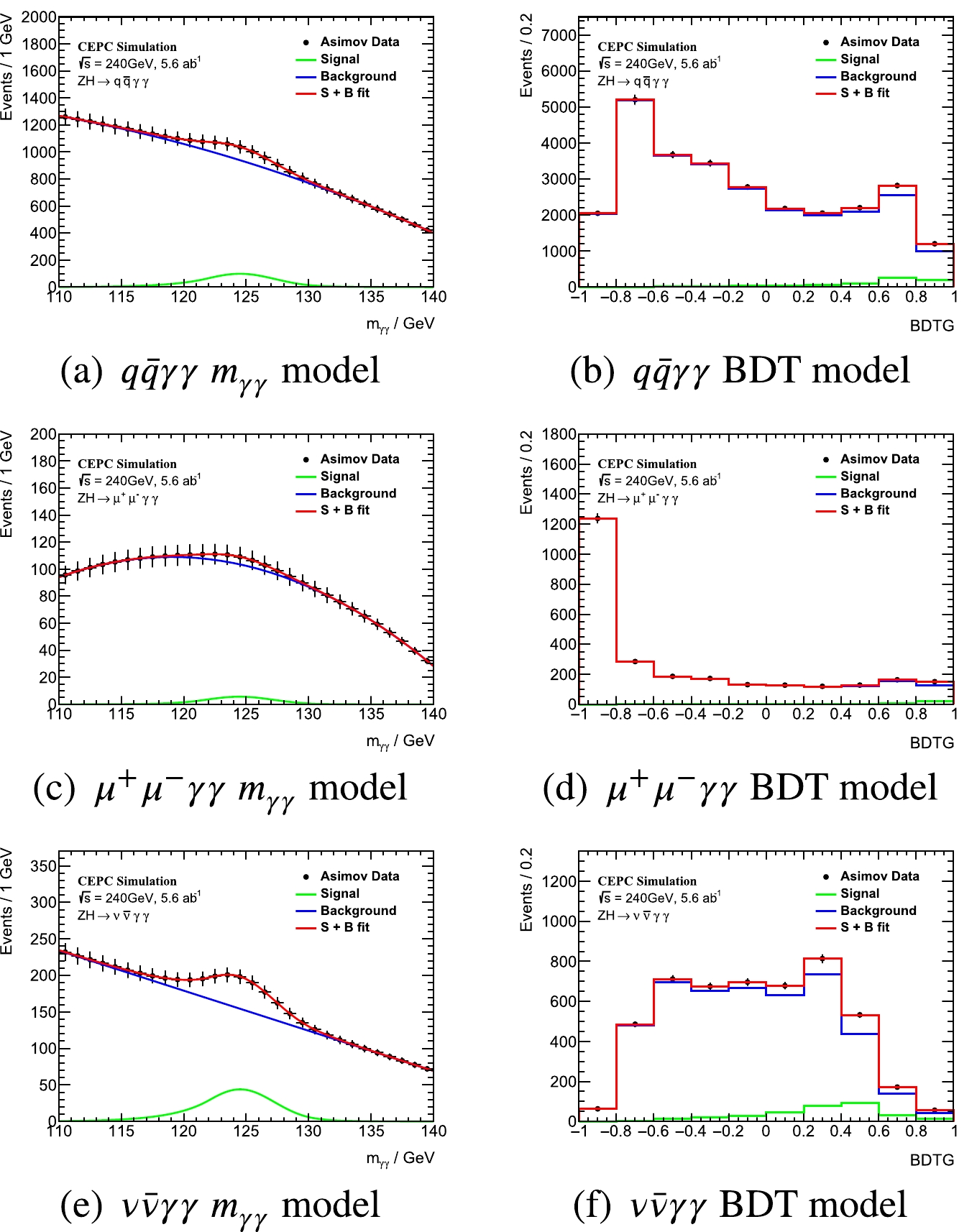
Figure 4. (color online) Combined fitting to the Asimov data in the three channels.
q\bar q\gamma \gamma 

{\mu ^ + }{\mu ^ - }\gamma \gamma 

\nu \bar \nu \gamma \gamma 

Theo 0.5% 0.005 - - Lumi 0.1% 0.001 0.001 0.001 photon eff 1% 0.019 0.020 0.020 PES 0.05% 0.001 <0.001 0.001 PER 0.05% <0.001 <0.001 <0.001 mH 5.9 MeV <0.001 <0.001 <0.001 BDT 0.006 0.006 0.007 Bkg. modeling 0.029 0.062 0.006 Table 9. Decoupled contributions from considered systematic uncertainties of the
(\sigma\times {\rm Br}) / (\sigma\times {\rm Br})_{\rm SM} measurement in the three channels. The 0.5% theoretical uncertainty was only considered in theq\bar q\gamma \gamma channel.5.6 ab−1 20 ab−1 \dfrac{\Delta_{\rm tot} }{(\sigma\times \rm Br)_{\rm SM} } 

\dfrac{\Delta_{\rm stat} }{(\sigma\times \rm Br)_{\rm SM} } 

\dfrac{\Delta_{\rm tot} }{(\sigma\times\rm Br)_{\rm SM} } 

\dfrac{\Delta_{\rm stat} }{(\sigma\times\rm Br)_{\rm SM} } 

q\bar q\gamma \gamma 

0.101 0.098 0.056 0.052 {\mu ^ + }{\mu ^ - }\gamma \gamma 

0.373 0.371 0.202 0.200 \nu \bar \nu \gamma \gamma 

0.130 0.127 0.071 0.067 Combined 0.079 0.077 0.046 0.040 Table 10. Expected precisions on
\sigma(ZH)\times {\rm Br}(H \to\gamma \gamma) from Asimov data fitting in the three channels and their combination. Results in 20 ab−1 were obtained by re-fitting the workspace with the scaled signal and background yields. The statistical precision includes the contribution from background modeling. -
Concerning the fitting of the
{m_{\gamma \gamma }} shape, the width of the signal peak is a direct connection between the measurement precision in theH\to \gamma\gamma channel and the ECAL resolution. Currently, a new detector design for CEPC is under development [12–14] in which the present Si-W sampling ECAL will be replaced by a homogeneous crystal ECAL. This new ECAL is expected to have an energy resolution of\sigma_{E}/E = 3\%/\sqrt{E} , which is almost five times higher than the sampling Si-W ECAL\sigma_{E}/E = 16\%/ \sqrt{E} \oplus 1\% [4]. This can facilitate photon detection and neutral meson (\pi^{0} ) reconstruction, and further contribute to the Higgs study in theH\to \gamma\gamma channel and flavor physics in the\pi^{0}\to \gamma\gamma final state, e.g.,B^0_{(s)} \to \pi^0 \pi^0 [31]. The jet energy resolution may not be significantly improved from this ECAL, given that the detector granularity is the dominant factor in PFA-based jet reconstruction.We performed a rough estimation in the
q\bar q\gamma \gamma channel according to the strategy followed in this work: to study the ECAL resolution impact on theH\to \gamma\gamma measurement. In the estimation, the selected photon was replaced by the truth photon with a smearing in its energy. Normally, the ECAL energy is approximated as:\begin{equation} \frac{\sigma_{E}}{E} = A \oplus \frac{B}{\sqrt{E}} \oplus \frac{C}{E}, \end{equation}

(6) where A is the constant term, e.g., the energy leakage and readout threshold; B represents the stochastic term from photoelectron statistics and depends on the sensitive material; and C comes from the electronic noise. Presently, the noise term C is expected to be 0, and the constant term A is expected to be at the level of 1%. The photon energy is smeared with the stochastic term B varying from 1% to 35%. Figure 5 shows a comparison between the
{m_{\gamma \gamma }} shape from the full simulation and two smearing points, i.e., 3% and 16%. The jet performance is maintained consistent with the baseline Si-W sampling ECAL, assuming there is no impact from the new detector. The same selection criteria as in Sec. III were applied; the BDT was not employed in this simplified study to focus on the photon detection only, which is expected to present a 30% decrease, approximately, compared with the results in Sec. VII. A Gaussian function was used to describe the signal model from energy smearing. The 2-dimensional model was replaced with a 1-dimension{m_{\gamma \gamma }} model, and a similar unbinned maximum likelihood fitting was performed to extract the signal strength precision\delta\mu/\mu without systematic uncertainties. Considering that{m_{\gamma \gamma }} and BDT are independent, this simplification was expected to have little impact on the relative improvement. Figure 6 shows the relationship between energy resolution B and fitted precision\delta\mu/\mu . These points can be fitted with the following function:
Figure 5. (color online) Signal shape for the full simulated
H \to \gamma\gamma sample (blue) and for two samples with smeared photon energy (3% in red and 16% in green). The fitted signal widths were 2.81 GeV, 0.94 GeV, and 1.96 GeV respectively.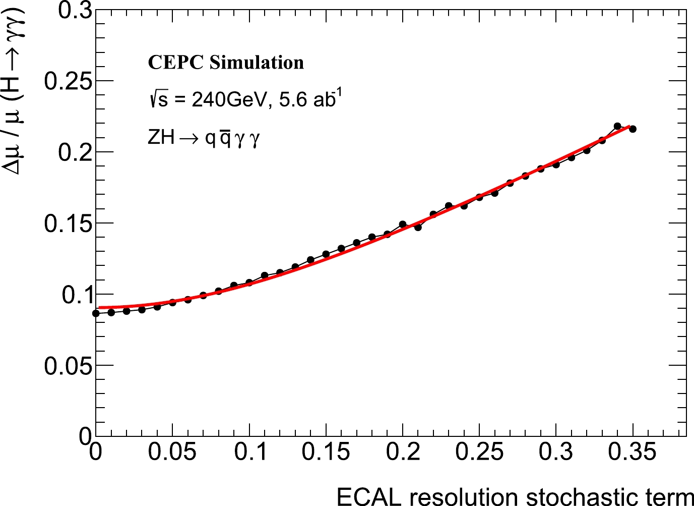
Figure 6. (color online) Signal strength measurement precision in the
ZH \to q\bar q\gamma \gamma channel as a function of the stochastic term in ECAL resolution from a fast analysis. The points were fitted using Eq. (7).\begin{equation} \frac{\delta \mu}{\mu} = p_{0} \oplus (p_{1}\times B), \end{equation}

(7) where
p_{0} andp_{1}\times B represent the contributions from the constant and stochastic terms, respectively. According to this relation, the homogeneous ECAL achieves a 28% improvement in the statistical precision of signal strength measurement. Moreover, a "critical point" can be defined: the two components in resolution equally contribute to\delta\mu/\mu , i.e.,p_{0}=p_{1}\times B . When the constant term A was fixed to 1%, the critical point for B, within this definition, was 14%. This indicates that the constant term in resolution would become the dominant contribution at the new ECAL design point with B = 3%. The scanning of a series of constant terms and the corresponding balanced stochastic terms are shown in Fig. 7.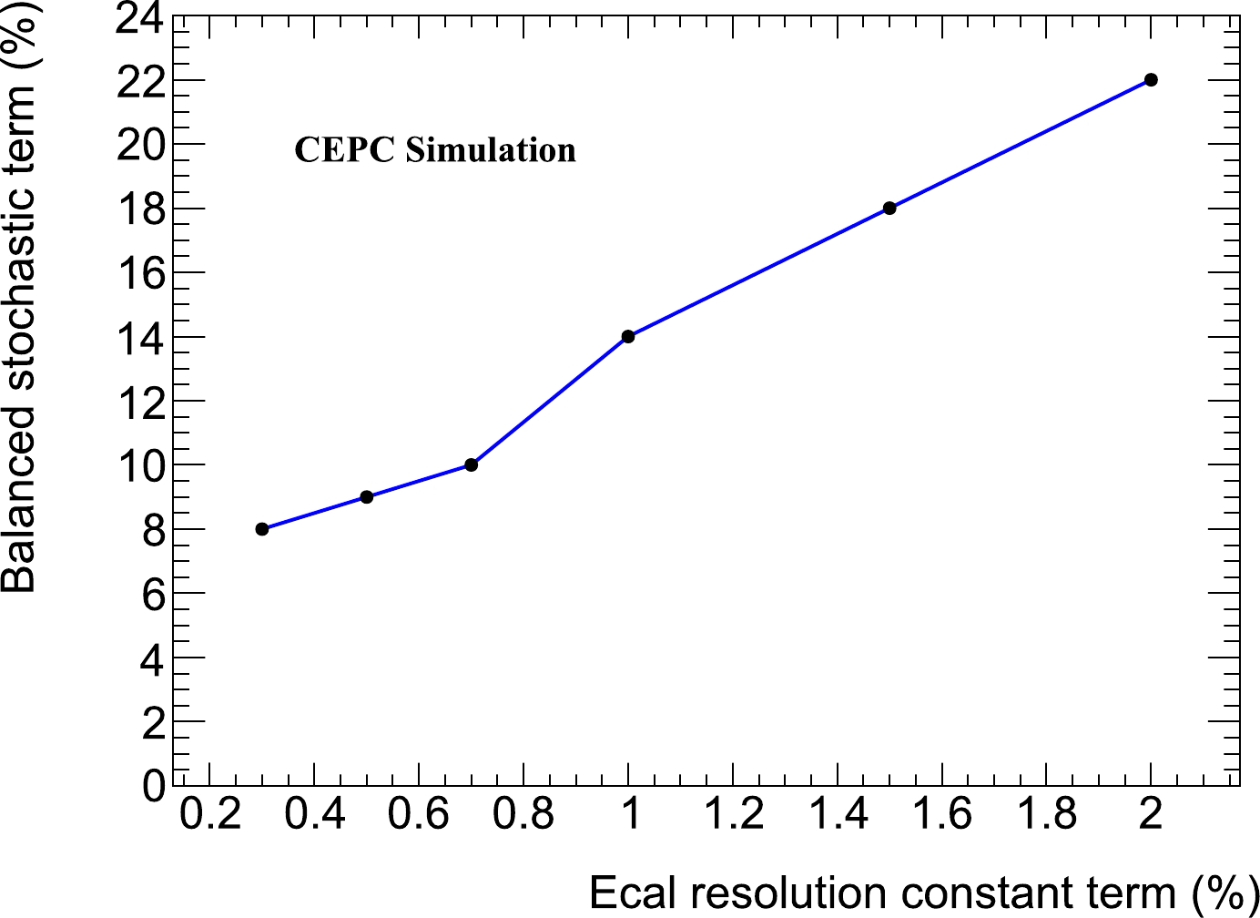
Figure 7. (color online) Balanced ECAL stochastic resolution points with different configurations of the constant term.
-
This paper reports on the expected precision for the measurement of the cross section times branching ratio in the CEPC via
ZH\to q\bar q\gamma \gamma ,ZH \to{\mu ^ + }{\mu ^ - }\gamma \gamma , andZH\to \nu \bar \nu \gamma \gamma channels. The physical events are reconstructed through CEPC-v4 detector simulation and selected according to a set of criteria. A BDTG was developed for further signal/background separation and used along with{m_{\gamma \gamma }} as discriminating variables in the maximum likelihood fitting when extracting the signal strength. We built a preliminary framework for systematic uncertainty analysis in the CEPC using nuisance parameters, and took several leading terms into account. With the scheduled integrated luminosity of 5.6 ab–1, a precision of 7.9% (7.7% stat.) is expected to be achieved at the CEPC. With 20 ab–1 data, this precision can be 4.6% (4.0% stat.). More mature results require further development of this framework and better knowledge of systematic terms in the CEPC. Meanwhile, the ECAL performance was studied by smearing photon energy resolution in theq\bar q\gamma \gamma channel. A direct relationship between the ECAL resolution and\sigma\times {\rm Br} precision is foreseen. -
The authors would like to thank the CEPC software group for the technical support of simulation and reconstruction packages, as well as the CEPC physics group for valuable discussions.
-
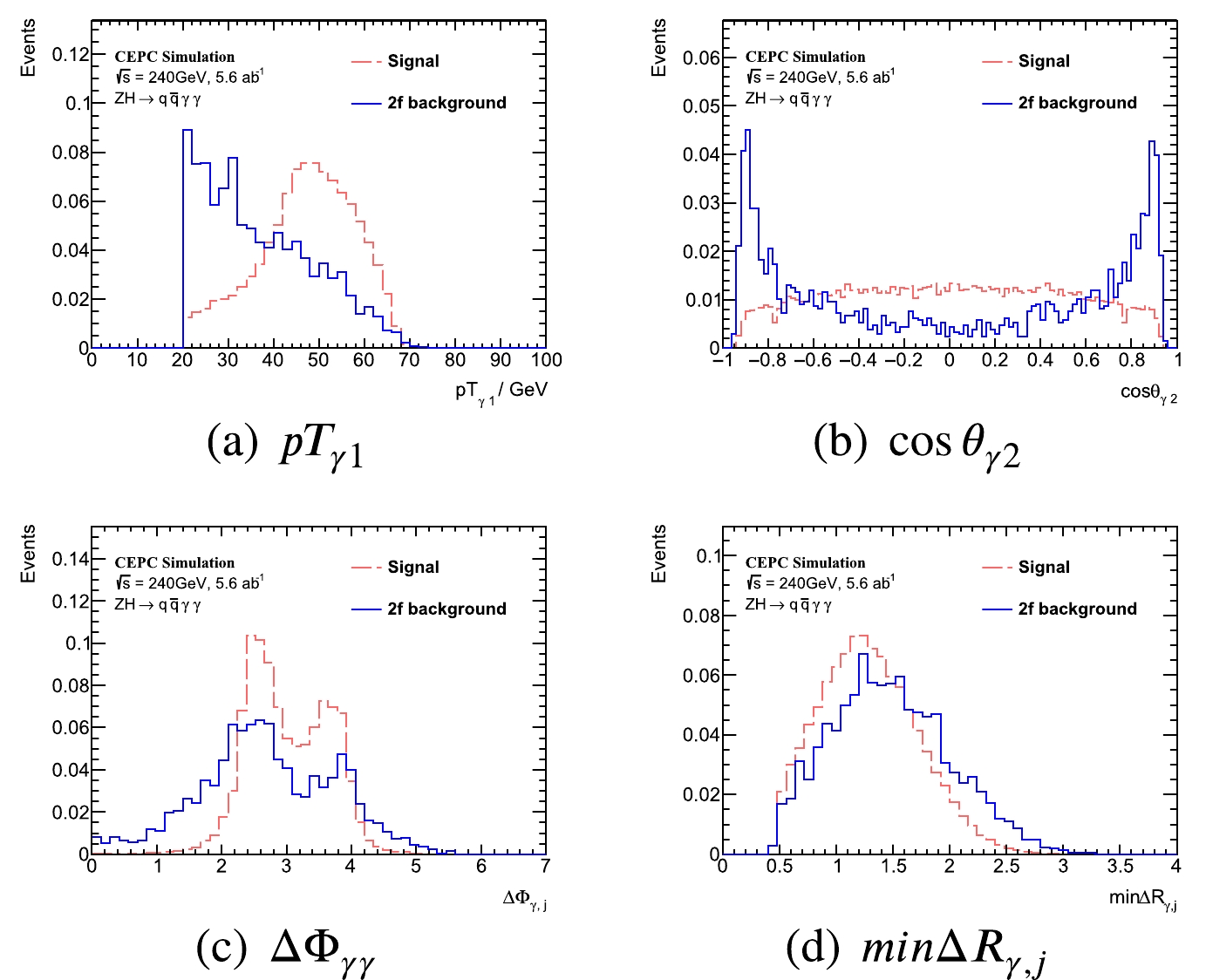

Figure A1-1. (color online) Training variables in
q\bar q\gamma \gamma channel. The signal and background yields are normalized.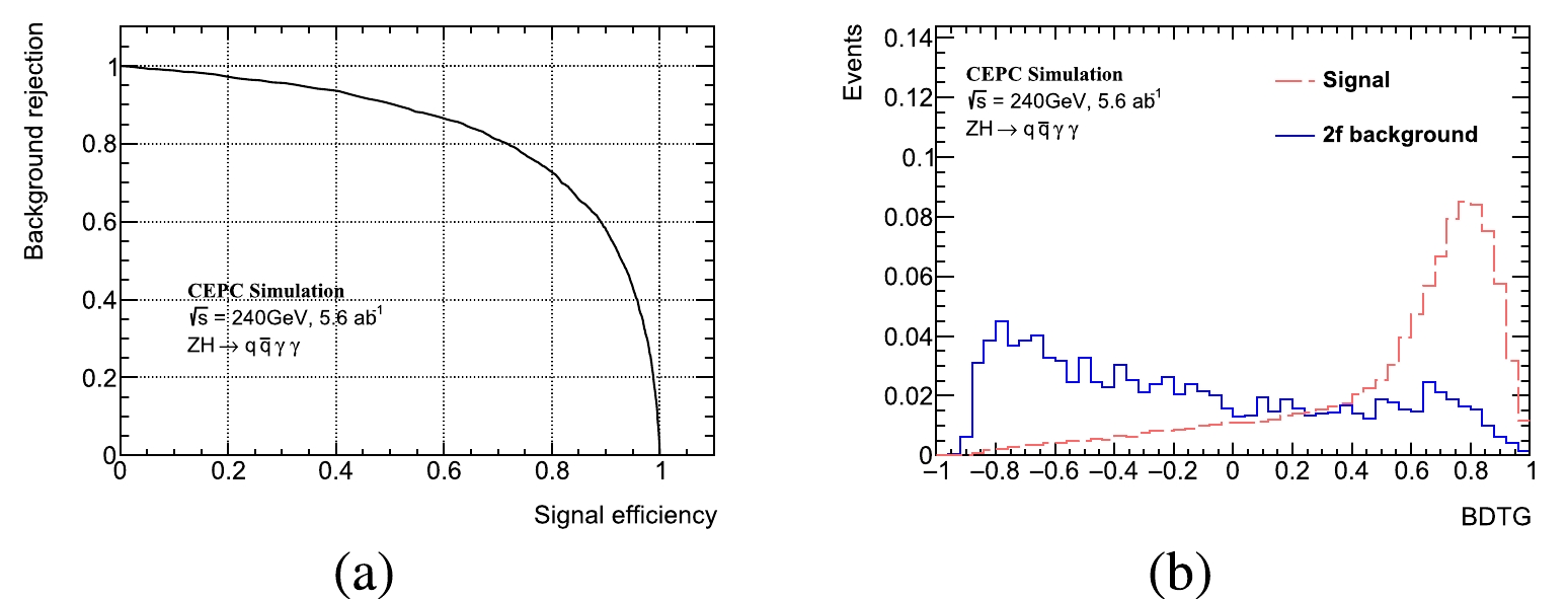
Figure A2. (color online) The ROC curve (left) and output BDTG distribution (right) in
q\bar q\gamma \gamma channel.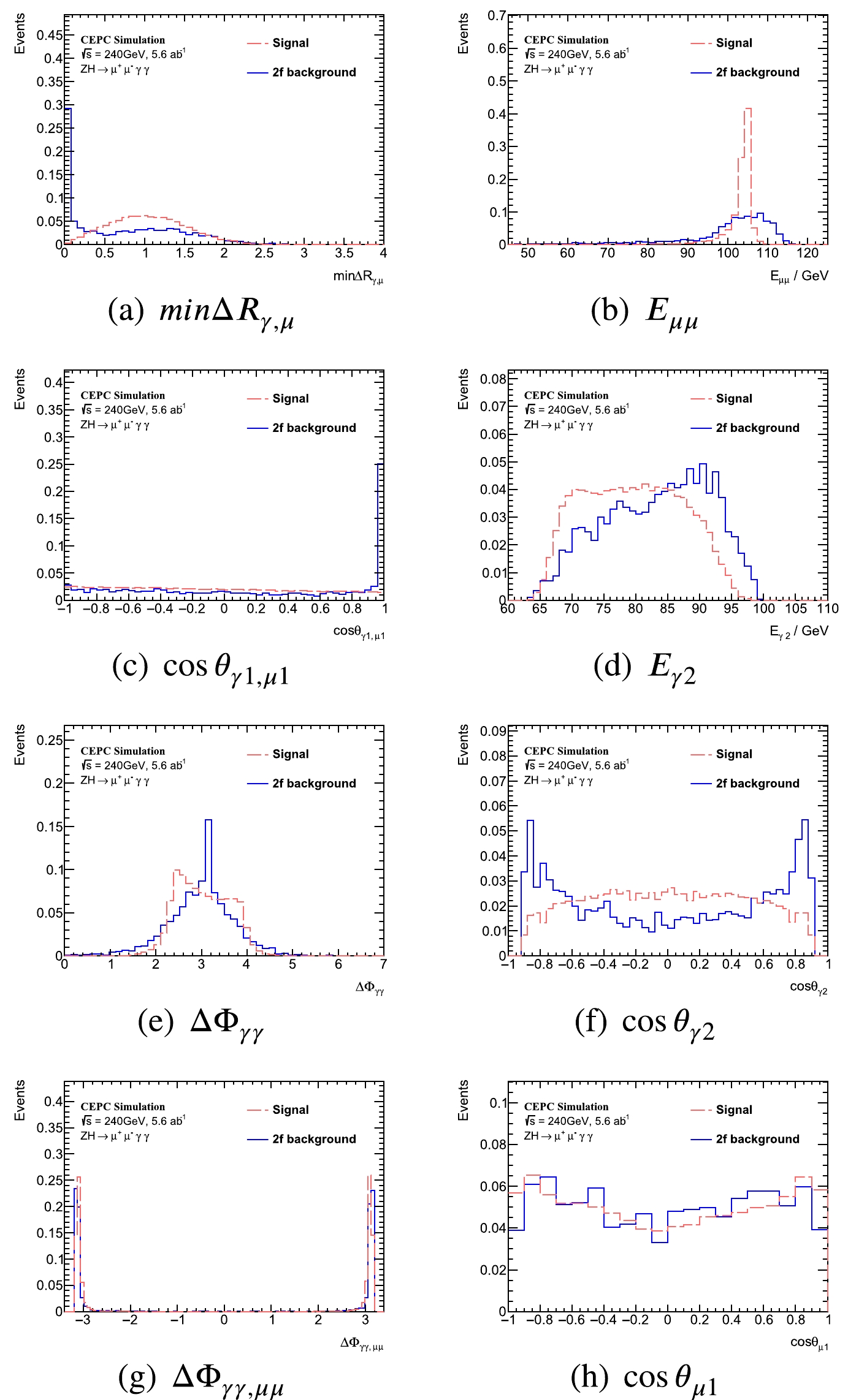
Figure A3. (color online) Training variables in
{\mu ^ + }{\mu ^ - }\gamma \gamma channel. The signal and background yields are normalized.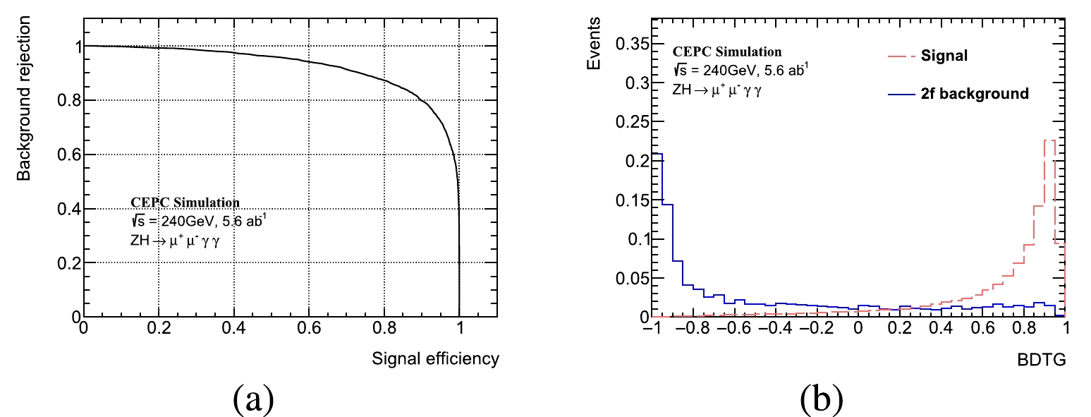
Figure A4. (color online) The ROC curve (left) and output BDTG distribution (right) in
{\mu ^ + }{\mu ^ - }\gamma \gamma channel.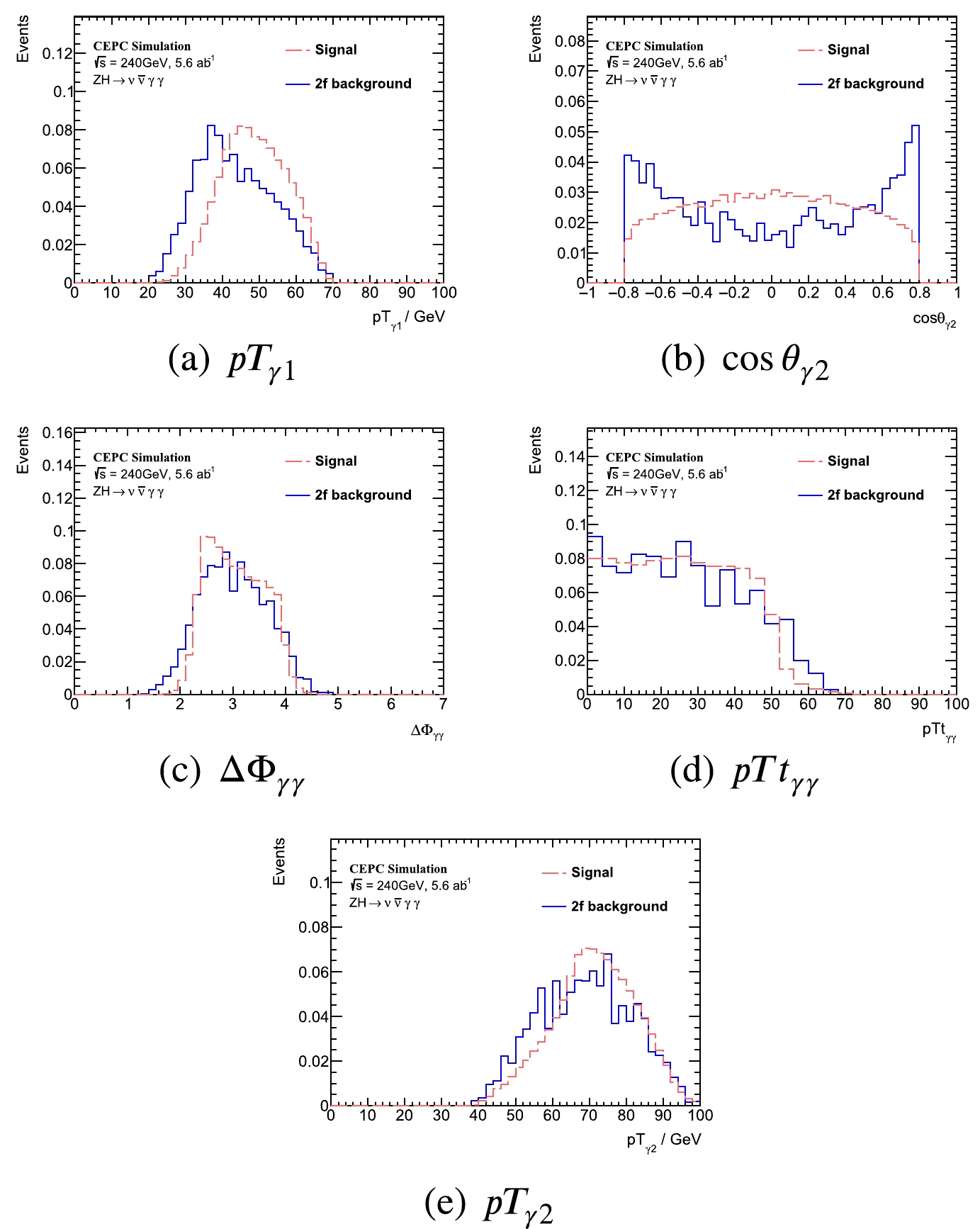
Figure A5. (color online) Training variables in
\nu \bar \nu \gamma \gamma channel. The signal and background yields are normalized.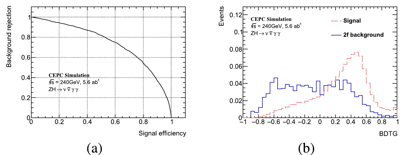
Figure A6. (color online) The ROC curve (left) and output BDTG distribution (right) in
\nu \bar \nu \gamma \gamma channel.q\bar q\gamma \gamma 

{\mu ^ + }{\mu ^ - }\gamma \gamma 

\nu \bar \nu \gamma \gamma 

1st order Exp. 0.941 5.423 3.786 2nd order Exp. 0.610 2.035 3.435 1st order Poly. 0.644 4.321 7.399 2nd order Poly. 0.600 3.758 3.439 1st order Chebyshev 0.644 4.321 3.320 2nd order Chebyshev 0.596 1.789 3.411 Table A1. The
\chi^{2} /Ndof values for 6 considered models in the background modeling in 3 channels, including the first and second order exponential, polynomial and Chebyshev functions.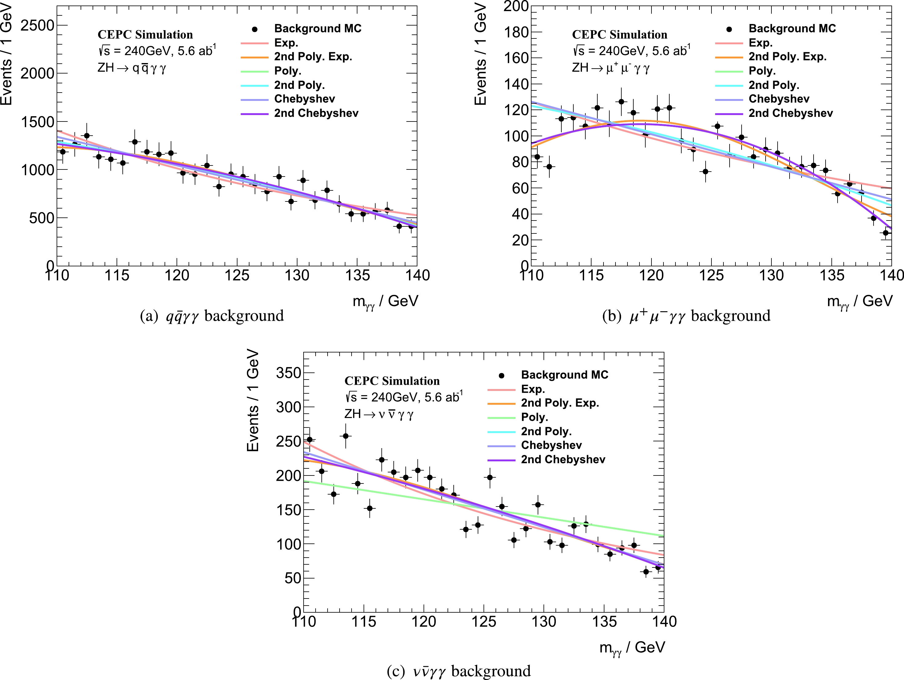
Figure A7. (color online) Tested functions for the background modeling. In All 3 channels the second order Chebyshev function gives the smallest
\chi^{2}/Ndof value. Detailed numbers are listed in Table A1.
Expected measurement precision of the branching ratio of the Higgs boson decaying to the di-photon at the CEPC
- Received Date: 2022-09-13
- Available Online: 2023-04-15
Abstract: This paper presents the prospects of measuring


 DownLoad: