Chromomagnetic and chromoelectric dipole moments of quarks in the reduced 331 model

The anomalous magnetic dipole moment (MDM) and the electric dipole moment are among the lepton properties that have attracted more interest in the experimental and theoretical areas. Currently, there is a discrepancy between the theoretical standard model (SM) prediction of the muon anomalous MDM and its experimental measurement, which might be a hint of new physics [1]. Moreover, any experimental evidence of an electric dipole moment would give a clear signal of new sources of $CP$ violation as the SM contributions are negligibly small. With the advent of the LHC, anomalous contributions to the $\bar{t}tg$ coupling have also become a focus of interest. In analogy with the lepton electromagnetic vertex $\bar\ell\ell\gamma$, the anomalous $\bar{q}qg$ coupling can be written as

where $\tilde{\mu}_q$ is the quark chromomagnetic dipole moment (CMDM) and $\tilde{d}_q$ is the quark chromoelectric dipole moment (CEDM), whereas $G^{\mu\upsilon}_a$ is the gluon field tensor and $T^a$ are the $SU(3)$ color generators. It is also customary to define the CMDM and CEDM in their dimensionless forms [2]

On the experimental side, the search for evidences of the anomalous top quark coupling $\bar{t}tg$ is underway at the LHC [2-4]. The most recent bounds on the top quark CMDM and CEDM were obtained by the CMS collaboration [4, 5], which managed to improve the previous bounds [2] by one order of magnitude. Thus, one would expect that tighter constraints on $\hat \mu_t$ and $\hat d_t$ could be set in the near future.

As far as the theoretical predictions are concerned, in the SM the CMDM is induced at the one-loop level or higher orders via electroweak (EW) and QCD contributions, whereas the CEDM can only arise up to the three-loop level [6-8]. The SM contributions to the on-shell $\hat\mu_t$ have already been studied in [9-11], and more recently the scenario with an off-shell gluon was studied in [12, 13] to address some ambiguities of previous calculations, particularly about the on-shell CMDM, which is divergent and meaningless in perturbative QCD. Given that both the top quark CMDM and CEDM could receive a considerable enhancement from new physics contributions, several calculations have been reported in the literature within the framework of extension theories such as the two-Higgs doublet models (THDMs) [14], the four-generation THDM [15], models with a heavy $Z'$ gauge boson [11], little Higgs models [16, 17], the minimal supersymmetric standard model (MSSM) [18], unparticle models [19], and vector like multiplet models [20]. In this study, we are interested in the contributions to the top quark CMDM and CEDM in the reduced 331 model [21].

The study of elementary particle models based on the $SU(3)_L \times U(1)_N$ gauge symmetry dates back to the 1970s, when it was not clear that Weinberg's $SU(2)_L \times U(1)_Y$ model was the right theory of electroweak interactions [22]. After the discovery of the Z and W gauge bosons, given that the electroweak gauge group is embedded into $SU(3)_L \times U(1)_N$, the so called 331 models [23, 24] became serious candidates to extend the SM and explain some issues with no answer, such as the flavor problem and the large splitting between the mass of the top quark and those of the remaining fermions. Several realizations of the 331 model have been proposed in the literature, which predict new fermions, gauge bosons, and scalar bosons. Their phenomenologies have been considerably studied [25-32].

The minimal 331 model [23, 24] requires a very large scalar sector that introduces three scalar triplets to give masses to the new heavy gauge bosons and one scalar sextet to endow the leptons with small masses. The complexity of this model has led to the appearance of alternative 331 models aimed to economize the scalar sector. In particular, the reduced 331 model (RM331) [21] only requires two scalar triplets, thereby being considerably simpler than the minimal version [33, 34]. In the RM331, the physical scalar states obtained after the symmetry breaking are two neutral scalar bosons only, with the lightest one being identified with the SM Higgs boson [35], and a doubly charged one. Unlike other 331 models, no singly charged scalar boson arises in the RM331 [36-38]. In the gauge sector, there is one new neutral gauge boson $Z'$, a new pair of singly charged gauge bosons $V^\pm$, and a pair of doubly charged gauge bosons $U^{\pm\pm}$. Similar to other 331 models, the RM331 also predicts three new exotic quarks. The original RM331 is strongly disfavored by experimental data [39], though it would still be allowed as long as left-handed quarks are introduced via a particular $SU(3)_L \times U(1)_N$ representation [40, 41], which in fact would give rise to flavor changing neutral current (FCNC) effects.

The contributions to the electron and muon anomalous MDM have been already studied in the RM331 [26] within another 331 realization [42]. As for the CMDM of quarks, there is only a previous calculation in the context of an old version of the 331 model [9], though such a calculation is limited to the on-shell case. However, given that the on-shell CMDM is infrared divergent in the SM [12], a calculation of the off-shell CMDM is mandatory. To the best of our knowledge, there is no calculation of the off-shell CMDM of quarks, let alone their off-shell CEDM, in 331 models. Furthermore, in the model studied in [9], the new contributions only arise in the gauge sector, whereas in the RM331 there are additional contributions from the neutral scalar bosons, which are absent in other 331 models.

In this paper, we present a study on the contributions of the RM331 to the off-shell CMDM and CEDM of the top quark. The manuscript is organized as follows. In Section II, we present a brief description of the RM331, with the Feynman rules necessary for our calculations presented in Appendix A. The analytical calculations of the new contributions to the dipole form factors of the $\bar{t}tg$ vertex are presented in Section III; our results in terms of Feynman parameter integrals and Passarino-Veltman scalar functions are presented in Appendix B. Section IV is devoted to a review of the current constraints on the parameter space of the model and the numerical analysis of the off-shell CMDM and CEDM of the top quark. Finally, in Section V, the conclusions and outlook are presented.

We briefly describe the main features of each sector of the RM331, with a focus only on those details relevant to our calculations.

As far as the scalar sector is concerned, the scalar potential is given by

where the scalar triplets transform as $\rho = \left(\rho^+,\rho^0,\rho^{++} \right)^T\sim$$(1,3,1)$ and $\chi = \left(\chi^-,\chi^{- -},\chi^0 \right)^T\sim(1,3,-1)$. To induce the spontaneous symmetry breaking (SSB), the neutral scalar bosons $\rho^0$ and $\chi^0$ develop non-zero vacuum expectation values (VEVs) under the shifting of the fields as

which leads to the following constraints

The $SU(3)_C \times SU(3)_L \times U(1)_N$ breaks down into the SM gauge group following the pattern

where $\upsilon_\rho$ can be identified with the SM Higgs VEV $\upsilon$. The left-over of SSB are two neutral scalar bosons and a pair of doubly charged ones $h^{\pm\pm}$, as explained below.

The mass matrix of the neutral scalar bosons in the $\left( R_\chi,R_\rho\right)$ basis is

where $t = \upsilon_{\rho}/\upsilon_\chi$. After diagonalization, the mass eigenstates in the limit $\upsilon_\chi\gg\upsilon_{\rho}$ are

with masses

where $\lambda_1$, $\lambda_2>0$ and $c_\beta\equiv \cos\beta \approx 1-\lambda_3^2\upsilon^2_{\rho}/(8\lambda_2^2 \upsilon_\chi^2)$. The SM Higgs boson h can be recovered in the $s_\beta\rightarrow 0$ limit, thus $h_1$ must be identified with the Higgs boson discovered at the LHC. Given that $m_{h}\simeq 125$ GeV, from Eq. (8), we obtain the relation $\lambda_1-\lambda_3^2/(4\lambda_2)\approx 0.26$ [1]. In the case $\lambda_2$, $\lambda_2<1$, and $\lambda_3<\lambda_2$, we obtain $m_{h_1}^2 = \lambda_1 \upsilon_{\rho}^2$, which recovers the SM case and thus $\lambda_1\approx 0.26$.

In the gauge sector, there are two new singly charged gauge bosons $V^\pm$, two doubly charged gauge bosons $U^{\pm\pm}$, and a neutral gauge boson $Z'$. They acquire their masses as follows. The would-be Goldstone bosons $\chi^\pm$ are eaten by the singly charged gauge bosons, whereas a linear combination of the doubly charged would-be Goldstone bosons $\rho^{\pm\pm}$ and $\chi^{\pm\pm}$ are absorbed by the doubly charged gauge boson $U^{\pm\pm}$. Also, the orthogonal combination of $\rho^{\pm\pm}$ and $\chi^{\pm\pm}$ gives rise to a physical doubly charged scalar boson pair $h^{\pm\pm}$. Finally, the would-be Goldstone boson $I_\chi$ becomes the longitudinal components of the $Z^\prime$ gauge boson. Thus, the masses of the new gauge bosons at leading order at $\upsilon_{\chi}$ are [43]

As far as the SM gauge bosons are concerned, the would-be Goldstone bosons $\rho^\pm$ and $I_\rho$ endow the Z and $W^\pm$ gauge bosons with masses, respectively.

The number of new fermions necessary to fill out the $SU(3)_L \times U(1)_N$ multiplets as well as their quantum numbers depend on the particular 331 model version. There are no new leptons in the RM331, but a new quark is required for each quark triplet. They transform as

with the numbers between parentheses representing the field transformations under the $SU(3)_C \times SU(3)_L \times U(1)_N$ gauge group, whereas $J_1$, $J_2$, and $J_3$ are the new exotic quarks with electric charges $Q_{J_{1,2}} = -4/3e$ and $Q_{J_{3}} = 5/3e$. Under this representation, the theory is anomaly free [40].

In the quark sector, the charged currents relevant for our calculations are given by the following Lagrangian

where the family index a runs over 1, 2, and 3, whereas i and l run over 1 and 2. Also $V_{\text{CKM}}^q = V_L^{u\dagger} V^d_L$ stands for the Cabibbo-Kobayashi-Maskawa matrix, with the mixing matrices $V^{u}_L$ ($V^{d}_L$) transforming the left-handed up (down) quarks flavor eigenstates into their mass eigenstates. It is assumed that the new quarks are given in their diagonal basis. Note that the doubly charged gauge boson $U^{\pm\pm}$ does not couple to the top quark.

Given that the $Z^\prime$ gauge boson couplings to the quarks are non-universal, flavor changing neutral currents (FCNCs) are induced at the tree level. The corresponding Lagrangian for the up quark sector reads

where the up quarks $u^\prime$ are in the flavor basis. It is evident that the above Lagrangian induces FCNC at the tree level after the rotation to the mass eigenstate basis.

In addition, the interactions between up quarks and the neutral scalar bosons arise from the Lagrangian

where $u'$ is an up quark triplet $u'^T = (u',c',t')$ and

with ${\bf{m}}^{u}$ being the quark mass matrix in the flavor basis [40]. After rotating to the mass eigenstate basis, only the terms proportional to ${\bf{m}}^{u}$ are diagonalized, whereas the remaining term gives rise to FCNC couplings, which can be written as

where

Through the parametrization reported in [44] for the ${\bf{V}}_{L,R}^{u,d}$ mixing matrices, it is possible to obtain numerical values for the entries of the ${\boldsymbol{\eta}}^{u,d}$ matrix. Under this framework, $m_{31}^u = 0$, $m_{32}^u = 0$, and $m_{33}^u = m_t$.

Apart from the pure SM contributions, at the one-loop level, there are new contributions to the CMDM of the top quark arising in both the gauge and scalar sectors of the RM331. The corresponding Feynman diagrams are depicted in Fig. 1. In the gauge sector, the new contributions arise from the neutral $Z'$ gauge boson and are induced by both diagonal and non-diagonal couplings. There is also a new contribution from the singly-charged gauge boson $V^\pm$, which is accompanied by the new exotic quark $J_3$. As already mentioned, the doubly-charged gauge boson $U^{\pm\pm}$ does not couple to the top quark, thus there is no contribution from this gauge boson to the top quark CMDM and CEDM. As for the scalar sector, there are new contributions from the neutral scalar bosons $h_1$ and $h_2$, which in fact are the novel contributions from the RM331 as they are absent in other 331 model versions. The SM-like Higgs boson $h_1$ yields new contributions arising from its FCNC couplings, which are induced at the tree-level and also from its diagonal coupling, which has a small deviation from its SM value. As for the new Higgs boson $h_2$, it also contributes via both diagonal and non-diagonal couplings. We would like to point out that such scalar contributions are absent in the 331 model studied in Ref. [9], where the on-shell CMDM of the top quark was calculated. Furthermore, as long as complex FCNC couplings are considered, there are non-vanishing contributions to the CEDM. This class of contributions has not been studied either in the context of 331 models.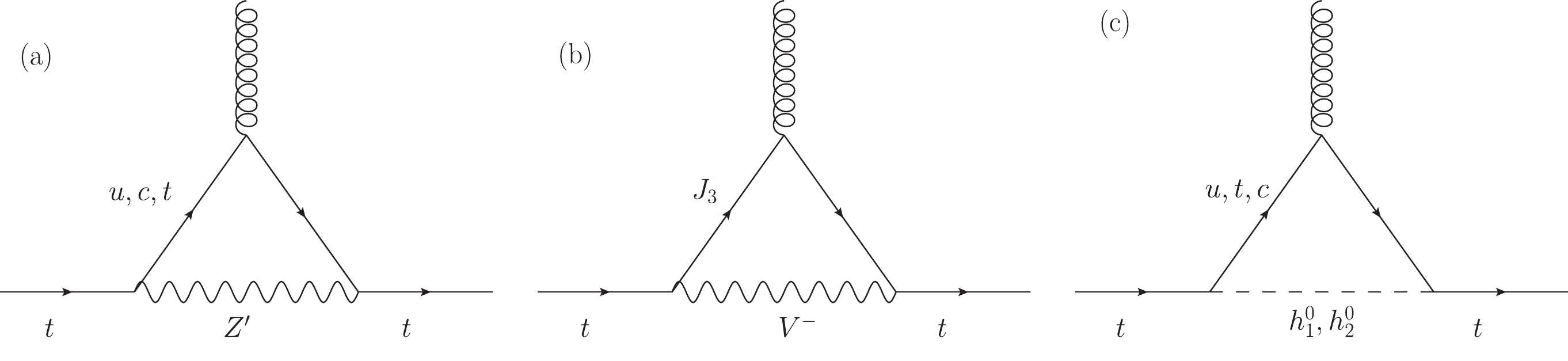

Figure 1.  New one-loop contributions of the RM331 to the CMDM and CEDM of the top quark in the unitary gauge. In the conventional linear $R_\xi$ gauge, there are additional Feynman diagrams in which the gauge bosons are replaced by their associated Goldstone bosons.

We are interested in the off-shell CMDM and CEDM of the top quark. Given that off-shell Green functions are not associated with an S-matrix element, they can suffer from issues such as being gauge non-invariant, gauge dependent, or ultraviolet divergent. In this context, the pinch technique (PT) was meant to provide a systematic approach to construct well-behaved Green functions [45], from which valid observable quantities can be extracted. It was later found that there is an equivalence at least at the one-loop level between the results found via the PT and those obtained through the background field method (BFM) via the Feynman gauge [46]. This provides a straightforward computational method to obtain gauge independent Green functions. It is thus necessary to verify whether the RM331 contributions to the CMDM and CEDM of quarks are gauge independent for $q^2\ne 0$. Nevertheless, from the Feynman diagrams in Fig. 1, note that the gauge parameter $\xi$ only enters the amplitudes of the Feynman diagrams (a) and (b) via the propagators of the gauge bosons and their associated would-be Goldstone bosons. Those types of diagrams have an amplitude that shares the same structure to those mediated by the electroweak gauge bosons Z and W in the SM, which are known to yield a gauge independent contribution to the CMDM for an off-shell gluon when the contribution of their associated would-be Goldstone bosons are added up. See for instance Ref. [12], where we calculated the electroweak contribution to the CMDM of quarks in the conventional linear $R_\xi$ gauge and verified that the gauge parameter $\xi$ drops out. Furthermore, the dipole form factors cannot receive contributions from self-energy diagrams, which are required to cancel gauge dependent terms appearing in the monopolar terms via the PT approach. Thus, both the CMDM and CEDM must be gauge independent for an off-shell gluon and hence valid observable quantities.

Below, we present the analytical results of our calculations in a model-independent way, from which the results for the RM331 and other SM extensions would follow easily. The corresponding coupling constants for the RM331 are presented in Appendix A. For loop integration, we used the Passarino-Veltman reduction method, and for completeness, our calculations were also performed through Feynman parametrization via the unitary gauge, which provides alternative expressions to cross-check the numerical results. The Dirac algebra and the Passarino-Veltman reduction were done in Mathematica with the help of Feyncalc [47] and Package-X [48].

We first consider the generic contribution of a new gauge boson V with the following interaction to the quarks

where the coupling constants $g_{V,A}^{Vqq'}$ are taken in general as complex quantities. By hermicity they should obey $g_{V,A}^{Vqq'} = g_{V,A}^{Vq'q*}$.

The above interaction gives rise to a new contribution to the quark CMDM and CEDM via a Feynman diagram similar to that of Fig. 1(a). The corresponding contribution to the quark CMDM can be written as

where we introduced the auxiliary variable $r_a = m_a/m_q$, and the ${\cal{V}}_{qq'}^V(q^2)$ function is presented in Appendix B in terms of Feynman parameter integrals and Passarino-Veltman scalar functions. The second term of the right-hand side stands for the first term with the indicated replacements. As for the contribution to the quark CEDM, it can arise as long as there are flavor changing complex couplings and is given by

where again the ${\cal{D}}_{qq'}^V(q^2)$ function is presented in Appendix B.

From Eqs. (17) and (18), we can straightforwardly obtain the contributions to the quark CMDM and CEDM of the neutral gauge boson $Z'$ and the singly charged gauge boson $V^\pm$ after replacing the coupling constants and the gauge boson masses.

Following the same approach described above, we next present the generic contribution to the quark CMDM and CEDM arising from FCNC mediated by a new scalar boson S, which arises from the Feynman diagram in Fig 1(c). We consider an interaction of the form

The above scalar interaction leads to the following contribution to the quark CMDM

whereas the corresponding contribution to the quark CEDM is given by

where the ${\cal{P}}_{qq'}^S(q^2)$ and $\widetilde{\cal{D}}_{qq'}^S(q^2)$ functions are presented in Appendix B.

From the above expression we can obtain the contribution of the new scalar Higgs boson of the RM331 as well as the contribution of the SM Higgs boson, which has tree-level FCNC couplings in the RM331.

We next address the numerical analysis. The coupling constants that enter the Feynman rules and are necessary to evaluate the CMDM and CEDM of the top quark [c.f. Eqs. (16) through (21)] are presented in Tables A1 and A2 of Appendix A. Note that these couplings depend on several free parameters, such as the mass parameter $m_{33}^u$, the VEV $\upsilon_\chi$, the parameters of the scalar potential $\lambda_2$ and $\lambda_3$, as well as the entries of the matrices ${\bf{V}}_L^u$, ${\bf{K}}_L$, and ${\boldsymbol{\eta}}^u$. To obtain an estimate of the contributions of the RM331 to the CMDM and CEDM of the top quark we need to discuss the most up-to-date constraints on these parameters from current experimental data.

Coupling	$g_V^{Vqq^\prime}$	$g_A^{Vqq^\prime}$
$Z^\prime \overline{t} t$	$\dfrac{1-2s_W^2}{2\sqrt{12 h_W}}$	$\dfrac{1-2s_W^2}{2\sqrt{12 h_W}}$
$Z\overline{t}q$	$\dfrac{s_W^2}{\sqrt{12 h_W}}\left(K_L\right)_{tq}$	$\dfrac{s_W^2}{\sqrt{12 h_W}}\left(K_L\right)_{tq}$
$V^- \overline{t}J_3$	$\sqrt{2}c_W (V^u_L)_{33}$	$\sqrt{2}c_W (V^u_L)_{33}$

Table A1.  Coupling constants for the interactions between gauge bosons and quarks in the RM331. We follow the notation of Lagrangian (16). Here $(K_L)_{tq}$ are entries of the complex mixing matrix ${\bf{K}}_{L}$, where the subscript q runs over u and c. This matrix is given in terms of the unitary complex matrix ${\bf{V}}^u_L$ that diagonalizes the mass matrix of up quarks and can be written as $(K_L)_{tq} = (V^u_L)^\ast_{tq}(V^u_L)_{qt}$. Here, $h_W = 1-4s_W^2$.

	$G_S^{Sqq^\prime}$	$G_P^{Sqq^\prime}$
$h_1\overline{t}t$	$\dfrac{m_t}{m_W} \left(c_\beta-\dfrac{\upsilon_{\rho}}{\upsilon_\chi}s_\beta\right)$	−
$h_1\overline{t}q$	$-\dfrac{s_\beta \upsilon_{\rho} m_{33}}{\upsilon_\chi\,m_W} \left(({\eta}^u)_{tq}+ ({\eta}^u)^\ast_{qt}\right)$	$-\dfrac{s_\beta \upsilon_{\rho} m_{33}}{\upsilon_\chi\,m_W} \left(({\eta}^u)_{tq}- ({\eta}^u)^\ast_{qt}\right)$
$h_2\overline{t}t$	$\dfrac{m_t}{m_W} \left(s_\beta-\dfrac{\upsilon_{\rho}}{\upsilon_\chi}c_\beta\right)$	−
$h_2\overline{t}q$	$\dfrac{c_\beta \upsilon_{\rho} m_{33}}{\upsilon_\chi\,m_W} \left(({\eta}^u)_{tq}+ ({\eta}^u)^\ast_{qt}\right)$	$\dfrac{c_\beta \upsilon_{\rho} m_{33}}{\upsilon_\chi\,m_W} \left(({\eta}^u)_{tq}- ({\eta}^u)^\ast_{qt}\right)$

Table A2.  Coupling constants for the interactions between scalar bosons and quarks necessary for the evaluation of the one-loop contributions to the CMDM and CEDM in the RM331. We follow the notation of Lagrangian (19). Here $({\eta}^u)_{tq}$ are entries of the complex mixing matrix ${\boldsymbol{\eta}}^u$, where the subscript q runs over u and c. This matrix is given in terms of the unitary complex matrices ${\bf{V}}^u_L$ and ${\bf{V}}^d_L$ that diagonalize the mass matrix of up quarks and can be written as $({\eta}^u)_{tq} = (V_L^u)_{q q}(V_R^u)^\ast_{t q}$ and $({\eta}^u)_{qt}^\ast = (V_L^u)^\ast_{t q}(V_R^u)_{q q}$ given that the matrix ${\boldsymbol{\eta}}^u$ is not symmetric.

As already mentioned, the mass parameter $m_{33}^u$ can be identified with the top quark mass [40], whereas the VEV $\upsilon_\chi$ determines the masses of the heavy gauge bosons and the heavy quark $J_3$. As for the mass of the new scalar boson $m_{h_2}$, it is determined by the parameters $\lambda_2$ and $\lambda_3$, along with the VEV $\upsilon_\chi$, which also determines the mixing angle $s_\beta$.

We will first discuss the current indirect constraints on the heavy neutral gauge boson masses. From the muon $g-2$ discrepancy, the constraint $\upsilon_\chi\geqslant 2$ TeV [41] was obtained, from which bounds on the heavy gauge boson masses follow. Nevertheless, there are also indirect constraints obtained through the experimental data on $B^0-\overline{B}^0$ oscillations. The RM331 contribution to $\Delta m_B$ arises from FCNC couplings mediated by the $Z'$ gauge boson and the $h_1$ and $h_2$ scalar bosons [40, 43]. Then, using the parametrization reported in [44], the experimental limit on $\Delta m_B$ leads to the following bounds: $m_{Z'}\gtrsim 3.3$ TeV, $m_{V^\pm}\gtrsim 0.33$ TeV and $m_{h_2}\gtrsim0.34$ TeV [40]. Similar limits have been imposed using the mass difference in the $K^0-\overline{K}^0$ and $D-\overline{D}^0$ systems [43]. In addition, the current experimental bounds on the masses of new neutral and charged heavy gauge bosons from collider searches are model dependent [1]. At the LHC, the ATLAS and CMS Collaborations have searched for an extra charged gauge boson $W'$ at $\sqrt{s} = 13$ TeV via the decay modes $W'\to \ell \nu_\ell$ [49, 50] and $W'\to qq'$. The most stringent bounds are obtained for a $W'$ gauge boson with SM couplings (sequential SM). The respective lower bounds on $m_{W'}$ are 6.0 TeV (5.1 TeV) for the $W'\to e \nu_e$ ($W'\to \mu \nu_\mu$) decay channel, whereas for the decay $W'\to q q'$, the corresponding bound is less stringent, of the order of $4$ TeV [51, 52]. As far as an extra neutral gauge boson $Z'$ is concerned, the search at the LHC at $\sqrt {s} = 13$ TeV via its decays into a lepton pair has been useful to impose the lower limit $m_{Z'}\geqslant 4.5,5$ TeV for a $Z'$ gauge boson model arising in the sequential SM and in an $E_6$-motivated Grand Unification model [53, 54]. In this context, it has been pointed out recently that the LHC might be able to constrain the mass of the heavy $Z'$ boson up to the $5$ TeV level in several 331 models [55-57]. Although these bounds are model dependent and rely on several assumptions, if we consider the conservative value of 5 TeV for the gauge boson masses, we obtain a lower constraint on $\upsilon_\chi$ of the order of 10 TeV. Thus, we will use this value in our analysis to be consistent with experimental constraints and limits from FCNC couplings.

As far as direct constraints on the mass of exotic quarks are concerned, the ATLAS and CMS Collaborations have used the $\sqrt{s} = 13$ TeV data to search for vector-like quarks with electric charge of $5/3$ via their decay into a top quark and a W gauge boson, with the final state consisting of a single charged lepton (muon or electron), missing transverse momentum, and several jets. A mass exclusion limit up to $1.6$ TeV is obtained depending on the properties of the vector-like quark [58-60]. We will thus use $m_{J_3} = 2$ TeV to be consistent with the experimental bound.

According to Eq. (8), the mass of the SM-like Higgs boson receives new corrections through the $\lambda_2$ and $\lambda_3$ parameters. As discussed above, the SM case is recovered when $\lambda_1\approx0.26$ and $\lambda_3<\lambda_2<1$. Thus, the new corrections to $m_{h_1}$ must lie within the experimental error of the SM Higgs boson mass $m_h = 125.10\pm 0.14$ GeV [1]. This allows constraining the $\lambda_2$ and $\lambda_3$ parameters, which in turn translates into constraints on $s_\beta$ and $m_{h_2}$ once the $\upsilon_\chi$ value is fixed. Again, we follow a conservative approach and only consider the experimental uncertainty in the Higgs boson mass, whereas theoretical uncertainties from higher order corrections are not taken into account. Note in Fig. 2 that the allowed regions in the planes $\lambda_2$ vs. $\lambda_3$ and $s_\beta$ vs. $m_{h_2}$ are consistent with the experimental error of the Higgs boson mass at 95% C.L. Note also that for a given $\lambda_2$, $\lambda_3$ must be approximately one order of magnitude below. In our calculations, we used $\lambda_2 = 0.9$ and $\lambda_3 = 0.06$, though there is no significant sensitivity of the top quark CMDM and CEDM to mild changes in the values of these parameters. In addition, we found that values ranging from $0.002$ to $0.013$ are allowed for $s_\beta$ provided that $\upsilon_\chi\geqslant 10$ TeV and $m_{h_2}\gtrapprox 300$ GeV, which is consistent with recent searches for new neutral scalar bosons at the LHC [1].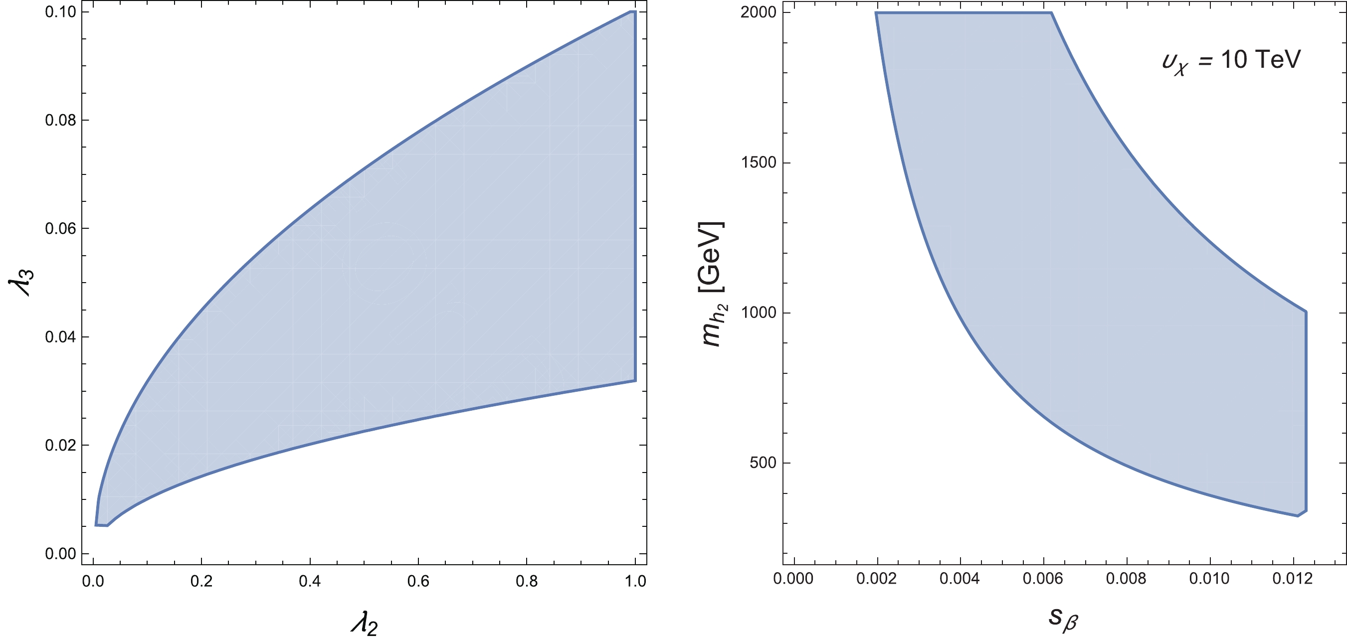

Figure 2.  (color online) Allowed areas in the planes $\lambda_3$ vs. $\lambda_2$ and $s_\beta$ vs. $m_{h_2}$ in agreement with the experimental error of the Higgs boson mass $m_h = 125.10\pm 0.14$ GeV [1] at 95% C.L. We consider $\lambda_1\approx 0.26$ and $\lambda_3<\lambda_2<1$, which yield the SM limit.

As for the mixing matrices, we can obtain the absolute values for the entries of the matrices ${\bf{V}}_L^u$, ${\bf{K}}_L$, and ${\boldsymbol{\eta}}^u$. The entries of the last matrix are given in terms of $\upsilon_\chi$, $s_\beta$, and the $m^q_{ij}$ matrix elements, and their values are obtained following the parametrization used in [44]. In general, ${\bf{K}}_L$ and ${\boldsymbol{\eta}}^u$ are expressed in terms of the entries of ${\bf{V}}_L^u$ and ${\bf{V}}_R^u$, i.e., the complex matrices that diagonalize the mass matrices of up quarks. These matrices can be assumed to be triangular. Then, using the experimental data on quark masses and the mixing angles, it is possible to obtain values of their entries [61]. It is also assumed that the only non-negligible mixing is that arising between the third and second fermion families. Furthermore, given that the $CP$ violation phases are expected to be very small, we follow a conservative approach and assume complex phases of the order of $10^{-3}$.

We present a summary of the values we used in our numerical evaluation in Table 1 .

Parameter	Value
$\left|(K_L)_{tc}\right|$	$6.4\times10^{-4}$
$\left|V^u_{33}\right|$	1
$\left|{\eta}^u_{tc}\right|$	$6.4\times 10^{-4}$
$\left|{\eta}^u_{ct}\right|$	$4.62\times 10^{-6}$
$m_{33}^u$	$m_t$
$\upsilon_\chi$	10 TeV
$s_\beta$	$10^{-2}$
$m_{h_2}$	300 GeV
$\phi_{{{\eta}}^u_{tc}} ,\; \phi_{{{\eta}}^u_{ct}}$	$10^{-3}$

Table 1.  Values of the parameters used in our evaluation of the CMDM and CEDM of the top quark in the RM331. For the entries of the matrices ${\bf{V}}_L^u$, ${\bf{K}}_L$, and ${\boldsymbol{\eta}}^u$, we used the values obtained in [40] using the parametrization of [44], where the mass parameter $m_{33}^u$ is identified with the top quark mass. We also used $\lambda_2$ and $\lambda_3$ values allowed by the experimental error in the Higgs boson mass and assumed that the only non-negligible mixing is that arising between the third and second fermion families.

As already mentioned, in the RM331 there are new contributions to the off-shell top quark CMDM $\mu_t(q^2)$ arising from the heavy gauge bosons $Z'$ and $V^\pm$ as well as the neutral scalar bosons $h_1$ and $h_2$. Below we will use the notation $A_{BC}$ for the contribution of particle A due to the $ABC$ coupling. Thus, for instance, $Z'_{tc}$ will denote the contribution of the loop with the $Z'$ gauge boson due to the $Z't c$ coupling. Given that we would like to assess the magnitude of the new physics contributions to $\hat \mu_t(q^2)$, we will extract the pure SM contributions from our calculations. Thus, apart from the contribution due to the tree-level FCNCs of the SM-like Higgs boson $h_1$, we only consider the contribution arising from the small deviation of the diagonal coupling $h_1tt$ from the SM $htt$ coupling. This contribution will be denoted by $\delta{h_1}_{tt}$.

We will examine the behavior of the CMDM of the top quark as a function of $\|q\|\equiv \sqrt{|q^2|}$, where q is the gluon four-momentum. In the left plot of Fig. 3 we show the real part of the partial contributions to $\hat\mu_t(q^2)$ as a function of $\|q\|$ for the parameter values in Table 1, whereas the real and imaginary parts of the total contribution are shown in the right plot. In general, there is little dependence of ${\rm{Re}}\left[\hat\mu_t(q^2)\right]$ on $\|q\|$, except for the $\delta{h_1}_{tt}$, $h_{2tt}$, and $h_{2tc}$ contributions, which have a change sign. Note also that the $V^\pm_{tJ_3}$ contribution is the largest one, whereas the remaining contributions are negligible, with the ${h_1}_{tc}$ contribution being the smallest one. Thus, the curve for the real part of the total contribution seems to overlap with that of the $V^\pm_{tJ_3}$ contribution, though the former shows a small peak at $\|q\|\simeq 2 m_t$. This can be explained by the peak appearing in the $\delta{h_1}_{tt}$ contribution, which can be as large as the ${V^\pm}_{tJ_3}$ contribution for $\|q\|\simeq 2 m_t$. We conclude that $\hat \mu_t(q^2)$ can have a real part of the order of $10^{-5}$.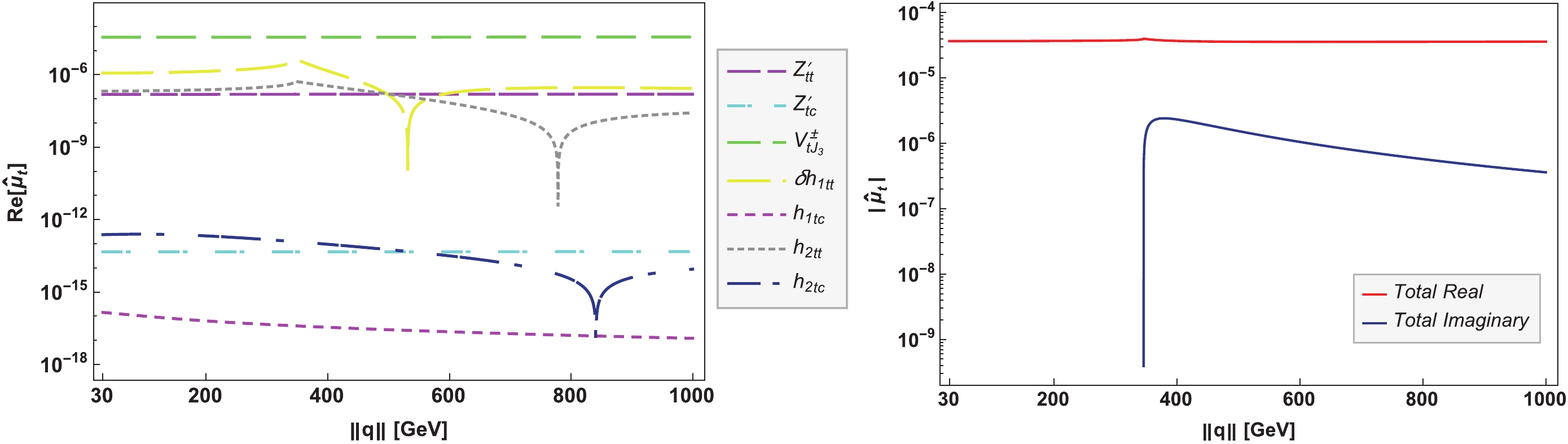

Figure 3.  (color online) Real part of the partial contributions of the RM331 to the top quark CMDM (left plot) as a function of $\|q\|\equiv\sqrt{|q^2|}$ for the parameter values in Table 1. The real and imaginary parts of the total contribution are shown in the right plot.

Concerning the imaginary parts of the partial contributions to $\hat\mu_t(q^2)$, they are several orders of magnitude smaller than the corresponding real parts. As observed in the right plot of Fig. 3, the imaginary part of the total contribution is negligible for $\|q\|\leqslant 2 m_t$ but increases up to approximately $10^{-6}$ around $\|q\| = 400$ GeV, where it starts to decrease up to one order of magnitude as $\|q\|$ increases up to 1 TeV.

Plots similar to those in Fig. 3 but depicting the behavior of $\hat\mu_t(q^2)$ as a function of $\upsilon_\chi$ for $\|q\| = 500$ GeV and the parameter values in Table 1 are shown in Fig. 4. In this case, note that the real parts of the partial contributions to $\hat\mu_t(q^2)$ show a variation of approximately one order of magnitude when $\upsilon_\chi$ increases from 10 TeV to 20 TeV. As already mentioned, the $V^\pm_{tJ_3}$ contribution yields the bulk of the total contribution to $\hat \mu_t$, whose imaginary part is slightly larger than its real part. Therefore, both real and imaginary contributions of the RM331 to the top quark CMDM can be as large as $10^{-5}$.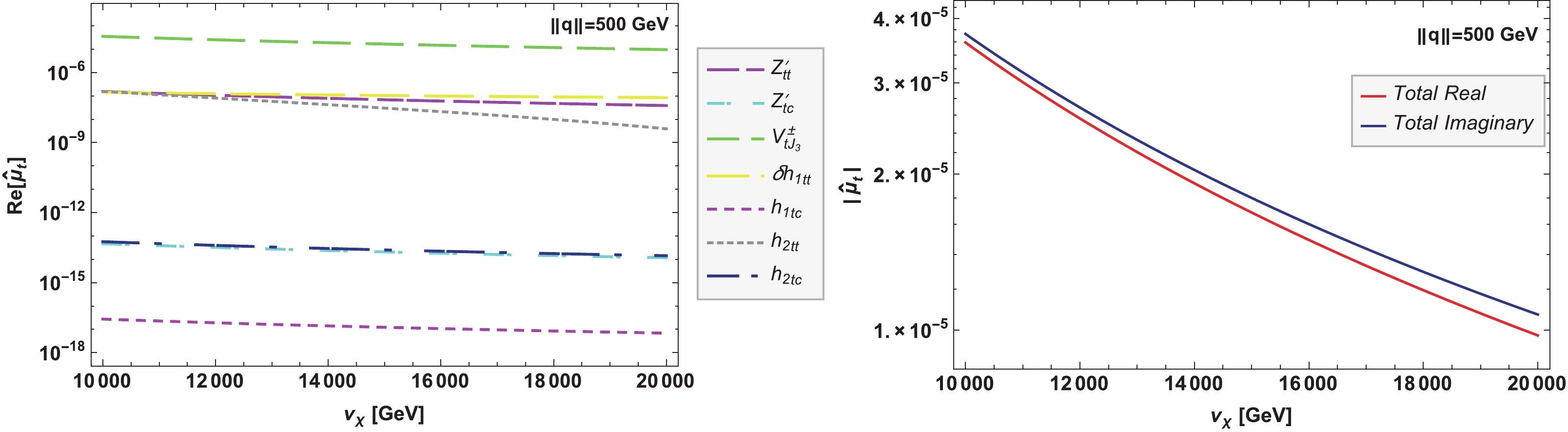

Figure 4.  (color online) Same plots as in Fig. 3 but for the contributions of the RM331 to the top quark CMDM as a function of $\upsilon_\chi$ for $\|q\|$ = 500 GeV. For the remaining parameters, we used the values in Table 1.

In summary, for $\upsilon_\chi\geqslant 10$ TeV, the real part of the new contribution of the RM331 to $\hat\mu_t(q^2)$ would be three orders of magnitude smaller than the real part of the SM electroweak contribution [12], whereas its imaginary part can be as large as its real part. In general, there is no appreciable variation in the magnitude of $\hat\mu_t$ for mild changes in the parameters listed in Table 1. Although $\hat\mu_t(q^2)$ can be of similar size to the SM electroweak prediction for $\upsilon_\chi\leqslant 10$ TeV, such values are disfavored by the current constraints on the heavy gauge bosons masses. Finally, note that the RM331 can render a contribution larger than the ones predicted by other extension models, where a new neutral Z gauge boson is predicted [11]. The real and imaginary parts of the top quark CMDM are of order $10^{-6}-10^{-7}$ and $10^{-10}-10^{-11}$ respectively in such models.

A potential new source of $CP$ violation can arise in the RM331 through the FCNC couplings mediated by neutral scalar bosons, which are proportional to the entries of the non-symmetric complex mixing matrix ${\boldsymbol{\eta}}^u$ [40], thereby allowing the presence of a non-zero CEDM, which is absent in other 331 models. Thus, it is a novel prediction of the RM331.

There are only two partial contributions to the top quark CEDM in the RM331. Thus, we only analyzed the behavior of the total contribution. Fig. 5 shows the contour lines of the real part (left plot) and the imaginary part (right plot) of $d_t(q^2)$ in the $\upsilon_\chi$ vs. $\|q\|$ plane for the parameter values listed in Table 1. We found that the new scalar boson $h_2$ yields the dominant contribution to $d_t(q^2)$, whose real (imaginary) part can be as large as $10^{-19}$ ($10^{-20}$), whereas the contribution from the $h_1$ scalar boson is three or more orders of magnitude below. Note also that the real part of $d_t(q^2)$ decreases as $\upsilon_\chi$ and $\|q\|$ increase, while the imaginary part remains almost constant. For $\|q\| \geqslant 600$ GeV, the RM331 contribution to the CEDM of the top quark is expected to be below the $10^{-20}$ level, which seems to be much smaller than the values predicted in other extension models [11], where the real and imaginary parts are of order $10^{-7}-10^{-8}$ and $10^{-12}-10^{-13}$, respectively. In the range 2 TeV $\leqslant\upsilon_\chi\lesssim$ 10 TeV, our results for $d_t(q^2)$ are enhanced by one order of magnitude, but as already mentioned, this interval is disfavored by current constraints.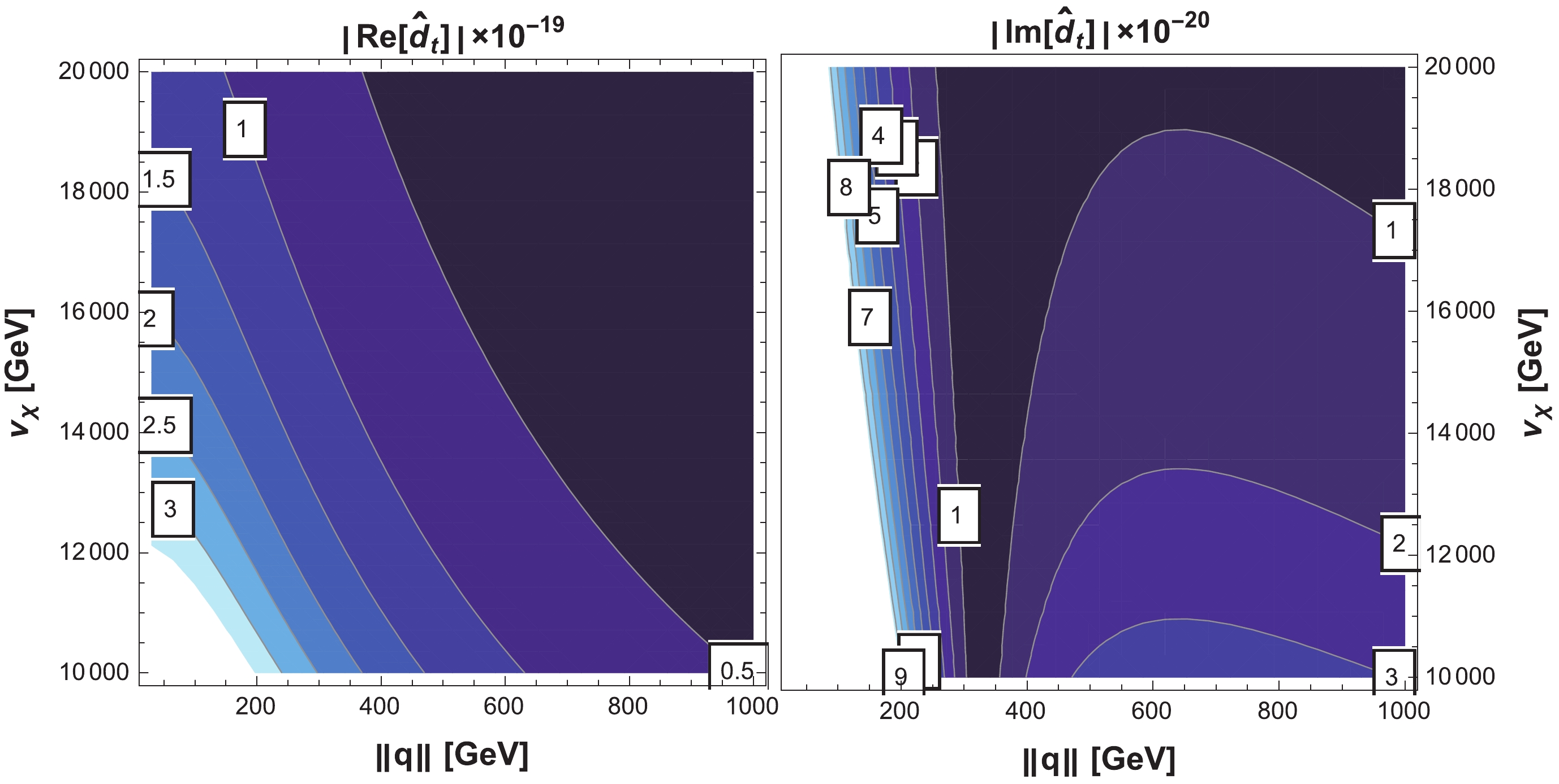

Figure 5.  (color online) Real part (left plot) and imaginary part (right plot) of the total contribution to the CEDM of the top quark in the RM331 in the plane $\upsilon_\chi$ vs. $\|q\|$. We used the parameter values in Table 1.

For comparison, a compilation of the predictions of several extension models of the top quark CMDM and CEDM for $q^2 = 0$ is presented in Table 2. We would like to stress that, to the best of our knowledge, there is no previous estimate of the top quark CEDM in 331 models. Note also that, although these values seem to be much larger than the results obtained for $q^2\neq0$ in the RM331, the dipole form factors are expected to decrease as $q^2$ increases. Such a behavior is indeed observed in the SM case [12], where the magnitude of $\hat{a}_t$ decreases as $\|q\|$ increases.

Model	$\hat{a}_t$	$\hat{d}_t$
SM	$10^{-2}$ [12, 13]
THDMs	$10^{-3}-10^{-1}$ [14]	$10^{-5}$ [14, 62]
4GTHDM	$10^{-2} -10^{-1}$ [15]	$10^{-5} - 10^{-4}$ [15]
331	$10^{-5}$ [9]
Technicolor	$10^{-2}$ [9]
Extra dimensions	$10^{-3}$ [9]
Little Higgs model	$10^{-6}$ [17]
MSSM	$10^{-1}$ [18]	$10^{-5}-10^{-4}$ [63]
Unparticle model	$10^{-2}$ [19]
Vector-like multiplets		$10^{-4}$ [20]

Table 2.  Predictions of the CMDM and CEDM of the top quark in several extension models at $q^2 = 0$.

We present a calculation of the one-loop contributions to the CMDM and CEDM, i.e., $\hat\mu_t(q^2)$ and $\hat d_t(q^2)$, of the top quark in the framework of the RM331, which is an economic version of the so-called 331 models with a scalar sector composed of two scalar triplets only. We consider the general case of an off-shell gluon, as it has been pointed out before, so that the QCD contribution to $\hat\mu_t(q^2)$ is infrared divergent and the CMDM has no physical meaning for $q^2 = 0$. We argue that the results are gauge independent for $q^2\ne 0$ and represent valid observable quantities given that the structure of the gauge boson contributions is similar to those arising in the SM. To the best of our knowledge, no previous calculations of the off-shell CMDM and CEDM of the top quark have been presented before in the context of 331 models.

Apart from the usual SM contributions, in the RM331, the CMDM of the top quark receives new contributions from two new heavy gauge bosons $Z'$ and $V^\pm$ as well as one new neutral scalar boson $h_2$, along with a new contribution from the neutral scalar boson $h_1$, which must be identified with the 125 GeV scalar boson detected at the LHC. This model also predicts tree-level FCNCs mediated by the $Z'$ gauge boson and the two neutral scalar bosons $h_1$ and $h_2$, which at the one-loop level can also give rise to a non-vanishing CEDM provided that there is a $CP$-violating phase. The analytical results are presented in terms of both Feynman parameter integrals and Passarino-Veltman scalar functions, which are useful to cross-check the numerical results.

We present an analysis of the region of the parameter space of the model consistent with experimental data and evaluate the CMDM and CEDM of the top quark for parameter values still allowed. It was found that the new one-loop contributions of the RM331 to the real (imaginary) part of $\hat \mu_t(q^2)$ are of the order of $10^{-5}$ ($10^{-6}$), which are larger than the predictions of other SM extensions [11], with the dominant contribution arising from the $V^\pm$ gauge boson, whereas the remaining contributions are considerably smaller. It was also found that there is little dependence of $\mu_t(q^2)$ on $\|q\|$ in the 30–1000 GeV interval for a mass $m_{V}$ of the order of a few hundreds of GeV. As far as the CEDM of the top quark is concerned, it is mainly induced by the loop with $h_2$ exchange and can reach values of the order of $10^{-19}$ for realistic values of the $CP$-violating phases. Such a contribution is smaller than the ones predicted by other SM extensions [11].

We acknowledge support from Consejo Nacional de Ciencia y Tecnología and Sistema Nacional de Investigadores. Partial support from Vicerrectoría de Investigación y Estudios de Posgrado de la Benemérita Universidad Autónoma de Puebla is also acknowledged.

We next present Tables A1 and A2 containing the coupling constants that enter the Feynman rules [26, 40, 43] that follow from Eqs. (16) and (19). These are necessary for the evaluation of the CMDM and CEDM of the top quark in the RM331.

In this appendix, we present the loop integrals appearing in Eqs. (17), (18), (20), and (21) in terms of Feynman parameter integrals and Passarino-Veltman scalar functions both for non-zero and zero $q^2$. We have verified that all the ultraviolet divergences cancel out. Furthermore, unlike the QCD contribution, all the contributions of the RM331 are finite for $q^2 = 0$.

The ${\cal{V}}_{qq'}^V(q^2)$ function in Eq. (17) can be written as

where $\Delta_V = u \left((u-1)+r_{V}^2\right)-r_{q^\prime}^2 (u-1)+{\hat q}^2 v (u+v-1)$, with ${\hat q}^2 = q^2/m_q^2$ and $r_a = m_a/m_q$.

For $q^2 = 0$, we obtain

As far as the $\widetilde{\cal{D}}_{qq'}^V(q^2)$ function in Eq. (18) is concerned, it is given by

which leads to

The ${\cal{P}}_{qq'}^S(q^2)$ function in Eq. (20) is

which for $q^2 =$ simplifies to

Finally, the loop function in Eq. (21) reads

which yields

We next present the results for the loop functions in terms of Passarino-Veltman scalar functions, which can be numerically evaluated by either LoopTools [64] or Collier [65], thereby enabling cross-checking the results. We introduce the following notation for two- and three-point scalar functions in the customary notation used in the literature:

for $a = V,S,q^\prime$ and $b = V,S$. We also define $\delta_b = 1-r_b$ and $\chi_b = 1+r_b$.

For non-zero $q^2$, the loop functions in Eqs. (17) and (18) are given by

and

As far as the results for $q^2 = 0$ are concerned, they read

and

The loop functions in Eqs. (20) and (21) are given by

and

For $q^2 = 0$, we obtain

and

To conclude the manuscript, we present the closed form solutions for the two-point Passarino-Veltman scalar functions appearing in the above calculations. The three-point scalar functions are too lengthy to be shown here.

where $\lambda(x,y,z) = x^2+y^2+z^2-2(xy-xz-yz)$. Note that the scale $\mu$ and pole $\epsilon$ of dimensional regularization cancel out in the final result.