


 Abstract
 HTML
HTML Reference
 Related
 PDF
PDF


-
The constituent quark model was initially proposed by Murray Gell-Mann [1] and George Zweig [2] for classification of hadrons formed from light quarks (u, d, s) and understanding their quantum numbers. It was later extended to hadrons containing heavy c or b quarks [3]. In addition to baryons containing a single heavy quark, the theory also predicts baryons comprising two heavy quarks. Such doubly heavy baryons provide a unique probe for quantum chromodynamics, the gauge theory of strong interactions. In 2017, the
$ {\rm{LHCb}} $ collaboration reported the first observation of the$ {{{{\varXi}^{++}_{cc}}}} $ baryon containing two charm quarks through the decay$ {{{{\varXi}^{++}_{cc}}}}{{\rightarrow }} {{{{\varLambda}^+_c}}}{{{K^-}}}{{{{\pi}^+}}}{{{{\pi}^+}}} $ [4].① The$ {{{{\varXi}^{++}_{cc}}}} $ state was later confirmed in the decay to$ {{{{\varXi}^+_c}}}{{{{\pi}^+}}} $ [5]. Its lifetime, mass and production cross-section were subsequently measured [6-8]. To date, no baryons containing one b and one c quark, or two b quarks, have been observed experimentally. An observation would enrich our knowledge of baryon spectroscopy and improve our understanding of the quark structure inside baryons.The ground-state baryons containing one b and one c quark, the
$ {{{{\varOmega}_{bc}^{0}}}} $ ($ b cs $ ),$ {{{{\varXi}_{bc}^{0}}}} $ ($ bcd $ ) and$ {{{{\varXi}_{bc}^{+}}}} $ ($ b c u $ ) states, have been considered within various theoretical models. Most studies predict the masses of the$ {{{{\varOmega}_{bc}^{0}}}} $ and$ {{{{\varXi}_{bc}^{0}}}} $ baryons to be between 6700 and 7200$ \;{\rm{MeV}}/{c^2} $ [9-25].The lifetime of the
$ {{{{\varOmega}_{bc}^{0}}}} $ baryon is predicted to be$ 0.22\pm0.04\;{\rm{ps}} $ [14], while the lifetime of$ {{{{\varXi}_{bc}^{0}}}} $ is predicted to be in the range of 0.09 to 0.28$ \;{\rm{ps}} $ [14, 23, 26, 27]. The production cross-section of the$ {{{{\varXi}_{bc}^{0}}}} $ baryon in proton-proton ($ pp $ ) collisions at a centre-of-mass energy$ \sqrt{s} = $ 14 TeV is expected to lie in the range between 19 to 39$\;{\rm{nb}} $ , derived from Ref. [28], in the$ {{{{\varXi}_{bc}^{0}}}} $ pseudorapidity ($ \eta $ ) range of$ 1.9 <\eta< 4.9 $ , depending on the required minimum value of the momentum component transverse to the beam direction ($ {{p_{\rm{T}}}} $ ) of the$ {{{{\varXi}_{bc}^{0}}}} $ particle. Recently, the$ {\rm{LHCb}} $ experiment found no significant$ {{{{\varXi}_{bc}^{0}}}} $ baryon signal in the predicted mass range using the$ {{{{\varXi}_{bc}^{0}}}}{{\rightarrow }} D^0 p{{{K^-}}} $ decay mode [29].This article reports the first search for the
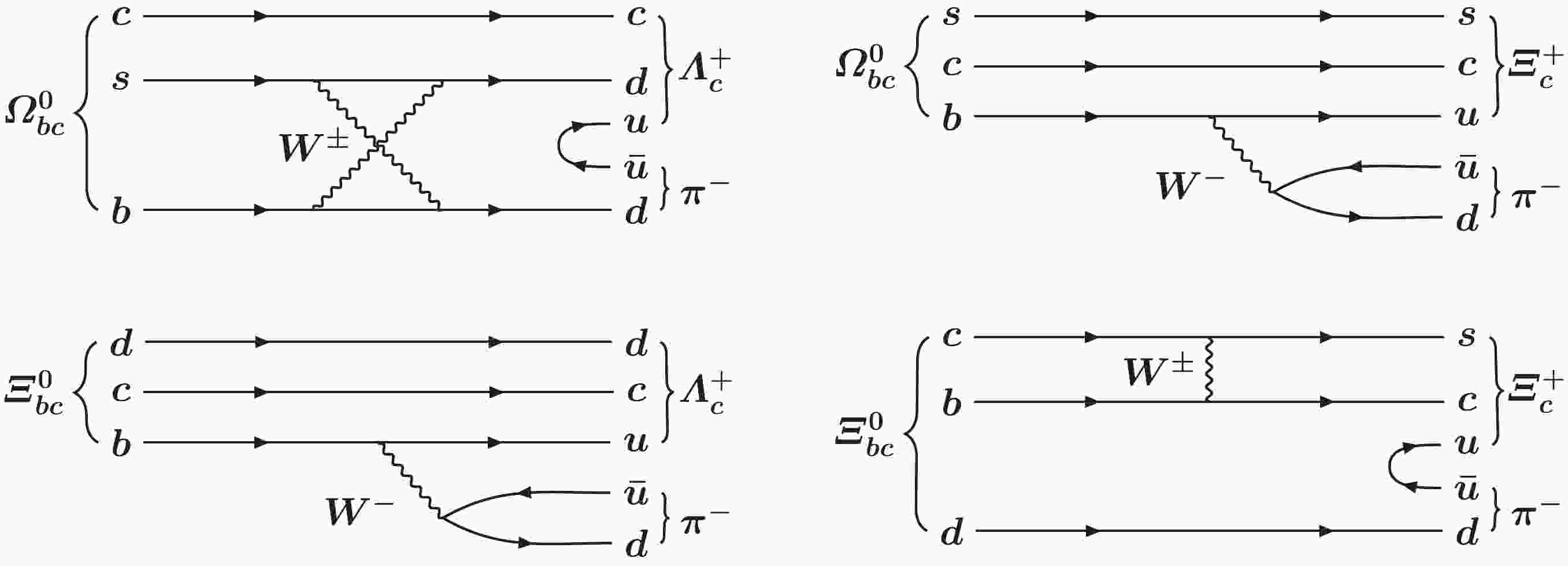
$ {{{{\varOmega}_{bc}^{0}}}} $ baryon and a new search for the$ {{{{\varXi}_{bc}^{0}}}} $ baryon, both via decay chains$ {{{{\varLambda}^+_c}}}{{{{\pi}^-}}} $ with$ {{{{\varLambda}^+_c}}}{{\rightarrow }}p{{{K^-}}}{{{{\pi}^+}}} $ or$ {{{{\varXi}^+_c}}}{{{{\pi}^-}}} $ with$ {{{{\varXi}^+_c}}}{{\rightarrow }}p{{{K^-}}}{{{{\pi}^+}}} $ in the$ {\rm{LHCb}} $ experiment. Examples of Feynman diagrams of the four signal decay modes are shown in Fig. 1. There are few theoretical predictions on the branching fractions of these decay modes. Ref. [30] predicts the branching fractions of the$ {{{{{{{{\varOmega}_{bc}^{0}}}}{{\rightarrow }}{{{{\varXi}^+_c}}}{{{{\pi}^-}}}}}}} $ and$ {{{{{{{{\varXi}_{bc}^{0}}}}{{\rightarrow }}{{{{\varLambda}^+_c}}}{{{{\pi}^-}}}}}}} $ decays to be$ 1.6\times10^{-7} $ and$ 3.0\times10^{-7} $ , respectively. However, uncertainties are not quoted. Inputs from experimental studies are necessary to deepen our understanding of the properties of$ {{{{\varOmega}_{bc}^{0}}}} $ and$ {{{{\varXi}_{bc}^{0}}}} $ baryons, and can provide valuable reference for future searches. Besides, the distinct experimental signatures of these decays make it promising to search for them in the$ {\rm{LHCb}} $ experiment considering the high detection efficiency of the$ {\rm{LHCb}} $ detector.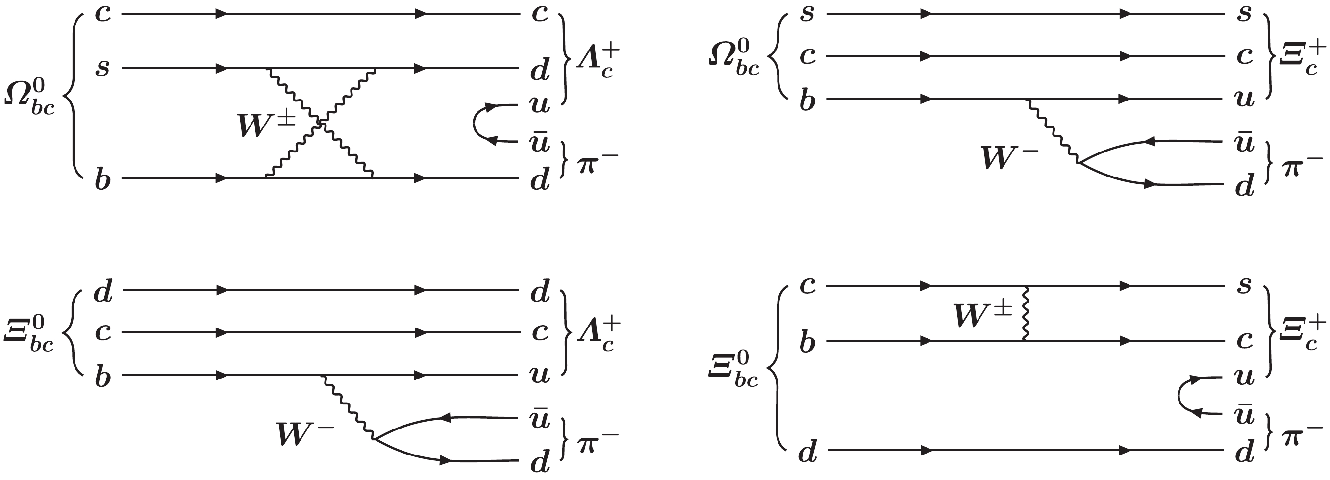
Figure 1. Examples of Feynman diagrams for the
$ {{{{{{{\varOmega}_{bc}^{0}}}}{{\rightarrow }}{{{{\varLambda}^+_c}}}{{{{\pi}^-}}}}}} $ ,$ {{{{{{{\varOmega}_{bc}^{0}}}}{{\rightarrow }}{{{{\varXi}^+_c}}}{{{{\pi}^-}}}}}} $ ,$ {{{{{{{\varXi}_{bc}^{0}}}}{{\rightarrow }}{{{{\varLambda}^+_c}}}{{{{\pi}^-}}}}}} $ and$ {{{{{{{\varXi}_{bc}^{0}}}}{{\rightarrow }}{{{{\varXi}^+_c}}}{{{{\pi}^-}}}}}} $ decays.The
$ {{{{\varOmega}_{bc}^{0}}}} $ and$ {{{{\varXi}_{bc}^{0}}}} $ baryons are not differentiated and are collectively denoted as$ {{{H_{bc}^{0}}}} $ hereafter, unless otherwise stated. The production cross-section times branching fraction of$H_{bc}^{0} \rightarrow \varLambda^+_c \pi^- $ $ { ({{{{{{H_{bc}^{0}}}} {{\rightarrow }}{{{{\varXi}^+_c}}}{{{{\pi}^-}}}}}})} $ decay is measured relative to that of the control channel$ {{{{{{{{\varLambda}^0_b}}}{{\rightarrow }}{{{{\varLambda}^+_c}}}{{{{\pi}^-}}}}}} ({{{{{{{\varXi}_{b}^{0}}}}{{\rightarrow }}{{{{\varXi}^+_c}}}{{{{\pi}^-}}}}}})} $ . This takes advantage of identical final-state particles and similar topology. The search is performed in the mass range between$ 6700 $ and$ 7300 \;{\rm{MeV}}/{c^2} $ using the$ pp $ collision data collected with the$ {\rm{LHCb}} $ experiment at$ {{\sqrt{s}}} = 13 \;{\rm{TeV}} $ , corresponding to an integrated luminosity of$ 5.2\;{\rm{f}}{{\rm{b}}^{ - 1}} $ . The$ {{{H_{bc}^{0}}}} $ baryons are reconstructed in the fiducial region of rapidity (y) between$ 2.0 $ and$ 4.5 $ and with$ {{p_{\rm{T}}}} $ between$ 2 $ and$ 20 \;{\rm{MeV}}/{c} $ . -
The
$ {\rm{LHCb}} $ detector [31, 32] is a single-arm forward spectrometer covering the$ {\rm{pseudorapidity}} $ range$ 2<\eta <5 $ , designed for the study of particles containing b or c quarks. The detector includes a high-precision tracking system consisting of a silicon-strip vertex detector surrounding the$ pp $ interaction region [33], a large-area silicon-strip detector located upstream of a dipole magnet with a bending power of approximately$ 4\;{\rm{Tm}} $ , and three stations of silicon-strip detectors and straw drift tubes [34] placed downstream of the magnet. The tracking system provides a measurement of the momentum, p, of charged particles with a relative uncertainty that varies from 0.5% at low momentum to 1.0% at 200$ \;{\rm{MeV}}/{c} $ . The minimum distance of a track to a primary$ pp $ collision vertex (PV), the impact parameter (IP), is measured with a resolution of$(15+29/{{p_{\rm{T}}}})\;\mu {\rm{m}}$ , where$ {{p_{\rm{T}}}} $ is in$ {\rm{MeV}}/{c} $ . Different types of charged hadrons are distinguished using information from two ring-imaging Cherenkov detectors [35]. Photons, electrons, and hadrons are identified by a calorimeter system consisting of scintillating-pad and preshower detectors, and an electromagnetic and a hadronic calorimeter. Muons are identified by a system composed of alternating layers of iron and multiwire proportional chambers [36]. The online event selection is performed by a trigger [37], which consists of a hardware stage, based on information from the calorimeter and muon systems, followed by a software stage, which applies a full event reconstruction. At the hardware trigger stage, events are required to have at least one hadron with$ {{E_{\rm{T}}}} $ larger than 3.5$ \;{\rm{GeV}} $ . The software trigger requires a two-, three-, or four-track secondary vertex with a significant displacement from any PV. At least one charged particle must have$ {{p_{\rm{T}}}} > 1.6 \;{\rm{MeV}}/{c} $ and be inconsistent with originating from any PV. A multivariate algorithm [38, 39] is used for the identification of secondary vertices consistent with the decay of a b hadron.Simulated samples are produced to model the effects of the detector acceptance and the imposed selection requirements. In the simulation,
$ pp $ collisions are generated using$ {\mathsf{PYTHIA}} $ [40, 41] with a specific$ {\rm{LHCb}} $ configuration [42]. A dedicated generator,$ {\mathsf{GENXICC2.0}} $ , is used to simulate the$ {{{H_{bc}^{0}}}} $ baryon production [43], with the mass and lifetime of the$ {{{H_{bc}^{0}}}} $ baryon set to$m({{{H_{bc}^{0}}}}) = 6900 $ $ \;{\rm{MeV}}/{c^2}$ and$ \tau({{{H_{bc}^{0}}}}) = 0.4\;{\rm{ps}} $ . Simulation samples with different mass (6700–7300$ \;{\rm{MeV}}/{c^2} $ ) and lifetime (0.2–0.4$ \;{\rm{ps}} $ ) hypotheses are obtained using a weighting technique with the generator level information on signal. Decays of unstable particles are described by$ {{\mathsf{EVTGEN}}} $ [44], in which final-state radiation is generated using$ {{\mathsf{PHOTOS}}} $ [45]. The interaction of the generated particles with the detector, and its response, is implemented using the$ {{\mathsf{GEANT4}}} $ toolkit [46, 47] as described in Ref. [48]. For the two control channels,$ {{{{{{{{\varLambda}^0_b}}}{{\rightarrow }}{{{{\varLambda}^+_c}}}{{{{\pi}^-}}}}}}} $ and$ {{{{{{{{\varXi}_{b}^{0}}}}{{\rightarrow }}{{{{\varXi}^+_c}}}{{{{\pi}^-}}}}}}} $ ,$ {\mathsf{PYTHIA}} $ is used to simulate the$ pp $ collisions and the production of the$ {{{{\varLambda}^0_b}}} $ and$ {{{{\varXi}_{b}^{0}}}} $ baryons. -
For both the
$ {{{H_{bc}^{0}}}} $ signal and the control channels, the$ {{{{\varLambda}^+_c}}}, {{{{\varXi}^+_c}}}{{\rightarrow }} p{{{K^-}}} {{{{\pi}^+}}} $ candidates are reconstructed from three charged particles identified as a proton, kaon and pion, respectively. The tracks are required to have good quality, and to be inconsistent with originating from any PV in the event. The tracks must also form a common vertex of good fit quality. The$ {{{{\varLambda}^+_c}}} $ ($ {{{{\varXi}^+_c}}} $ ) candidate is required to have an invariant mass in the range 2271–2301$ \;{\rm{MeV}}/{c^2} $ (2450–2488$ \;{\rm{MeV}}/{c^2} $ ), corresponding to approximately six times the$ {{{{\varLambda}^+_c}}} $ ($ {{{{\varXi}^+_c}}} $ ) mass resolution, and to be inconsistent with originating from any PV. In the sample of selected$ {{{{\varLambda}^+_c}}} $ ($ {{{{\varXi}^+_c}}} $ ) candidates, there is a sizable background contamination from decays of other particles, such as$ {{{D^+}}} $ ($ {{{D^+_s}}} $ ) decays to$ {{{K^-}}}{{{{\pi}^+}}}{{{{\pi}^+}}} $ ($ {{{K^-}}}{{{K^+}}}{{{{\pi}^+}}} $ ) with a charged pion (kaon) misidentified as a proton, and background from$ \phi{{{{\pi}^+}}} $ combinations where in$ \phi{{\rightarrow }}{{{K^-}}}{{{K^+}}} $ decays a kaon is misidentified as a proton. Such background candidates are rejected if the$ {{{K^-}}}{{{{\pi}^+}}}{{{{\pi}^+}}} $ ,$ {{{K^-}}}{{{K^+}}}{{{{\pi}^+}}} $ or$ {{{K^-}}}{{{K^+}}} $ invariant mass is consistent with the known$ {{{D^+}}} $ ,$ {{{D^+_s}}} $ or$ \phi $ mass [49], respectively, when a charged pion (kaon) hypothesis is assigned to the proton candidate.An additional charged particle identified as a pion and, with
$ {{p_{\rm{T}}}} $ greater than 0.2$ \;{\rm{MeV}}/{c} $ , is combined with the$ {{{{\varLambda}^+_c}}} $ ($ {{{{\varXi}^+_c}}} $ ) candidate to form an$ {{{H_{bc}^{0}}}} $ candidate. The$ {{{H_{bc}^{0}}}} $ candidates must have a vertex with good fit quality, a decay time larger than 0.05$ \;{\rm{ps}} $ , a$ {{p_{\rm{T}}}} $ greater than 2$ \;{\rm{MeV}}/{c} $ and a scalar sum of the$ {{p_{\rm{T}}}} $ of the final-state particles greater than 5$ \;{\rm{MeV}}/{c} $ . Furthermore, the$ {{{H_{bc}^{0}}}} $ candidates are required to be consistent with originating from a PV. To avoid contributions from duplicate tracks, the selected candidates are rejected if the angle between any pair of the final-state particle tracks with same charge is smaller than 0.5$ {{\rm{\,{mrad}}}} $ .A boosted decision tree (BDT) classifier [50, 51] implemented in the TMVA toolkit [52, 53] is used to further suppress combinatorial background. A simulated signal sample in the mass range 6846–6954
$ \;{\rm{MeV}}/{c^2} $ and a background sample formed by candidates in an upper mass sideband region (7500–9000$ \;{\rm{MeV}}/{c^2} $ ) are used to train the BDT classifier. Four different categories of variable are used as the BDT input. The first category exploits the non-zero lifetime of$ {{{H_{bc}^{0}}}} $ baryons and a displacement of their vertices from any PV in the event. The variables comprise the$ {\chi^2_{\rm{IP}}} $ of all final-state particles forming the$ {{{{\varLambda}^+_c}}} $ ($ {{{{\varXi}^+_c}}} $ ) and$ {{{H_{bc}^{0}}}} $ candidates with respect to their associated PV, where$ {\chi^2_{\rm{IP}}} $ is defined as the difference in the vertex-fit$ {\chi^2} $ of a given PV reconstructed with and without the particle under consideration, and the associated PV is the one with respect to which the$ {{{H_{bc}^{0}}}} $ candidate has the smallest$ {\chi^2_{\rm{IP}}} $ ; the sum of$ {\chi^2_{\rm{IP}}} $ of the four final-state particles; and$ {\chi^2} $ of the flight distance of the$ {{{{\varLambda}^+_c}}} $ ($ {{{{\varXi}^+_c}}} $ ) and$ {{{H_{bc}^{0}}}} $ candidates. The second category consists of kinematic variables, including$ {{p_{\rm{T}}}} $ of the final-state particles and the$ {{{{\varLambda}^+_c}}} $ ($ {{{{\varXi}^+_c}}} $ ) and$ {{{H_{bc}^{0}}}} $ candidates, and the angle between the$ {{{H_{bc}^{0}}}} $ momentum vector and the displacement vector pointing from the associated PV to the$ {{{H_{bc}^{0}}}} $ decay vertex. The third category comprises the vertex-fit$ {\chi^2} $ of the$ {{{{\varLambda}^+_c}}} $ ($ {{{{\varXi}^+_c}}} $ ) and$ {{{H_{bc}^{0}}}} $ candidates, and$ {\chi^2} $ of a kinematic fit [54] of the signal decay chain constraining the$ {{{H_{bc}^{0}}}} $ candidate to originate from the associated PV. The fourth category consists of identification variables of the final-state particles.The BDT threshold is chosen to maximize the figure of merit,
$ \varepsilon/(\dfrac{\alpha}{2} + \sqrt{B}) $ [55]. Here,$ \varepsilon $ is the selection efficiency of signal candidates determined from simulation, B is the expected background number in the signal mass region, and$ \alpha = 5 $ is the signal significance. This threshold is estimated using the signal sample simulated with the default mass and lifetime values. The same selection is applied to the control modes. -
To improve the resolution of the mass of the
$ {{{H_{bc}^{0}}}} $ candidates, the$ {{{{\varLambda}^+_c}}}{{{{\pi}^-}}} $ ($ {{{{\varXi}^+_c}}}{{{{\pi}^-}}} $ ) invariant mass is calculated after constraining the$ {{{{\varLambda}^+_c}}} $ ($ {{{{\varXi}^+_c}}} $ ) mass to its known value [49] and requiring the$ {{{H_{bc}^{0}}}} $ candidate to be consistent with originating from its associated PV. The obtained invariant mass distributions of$ {{{H_{bc}^{0}}}} $ candidates,$ m({{{{\varLambda}^+_c}}}{{{{\pi}^-}}}) $ and$ m({{{{\varXi}^+_c}}}{{{{\pi}^-}}}) $ , are shown in Fig. 2. To search for the$ {{{H_{bc}^{0}}}} $ signals, the mass distributions are fitted using an unbinned maximum-likelihood fit. A double-sided Crystal Ball function [56] is used to model the signal, with tail parameters fixed from simulation, and the peak position and width allowed to vary in the fit. The background shape is interpolated from a double-exponential fit to a lower (6100–6650$ \;{\rm{MeV}}/{c^2} $ ) and an upper (7500–9000$ \;{\rm{MeV}}/{c^2} $ ) sideband region of the$ {{{{\varLambda}^+_c}}}{{{{\pi}^-}}} $ ($ {{{{\varXi}^+_c}}}{{{{\pi}^-}}} $ ) mass distribution. No significant excess is observed across the searched mass range.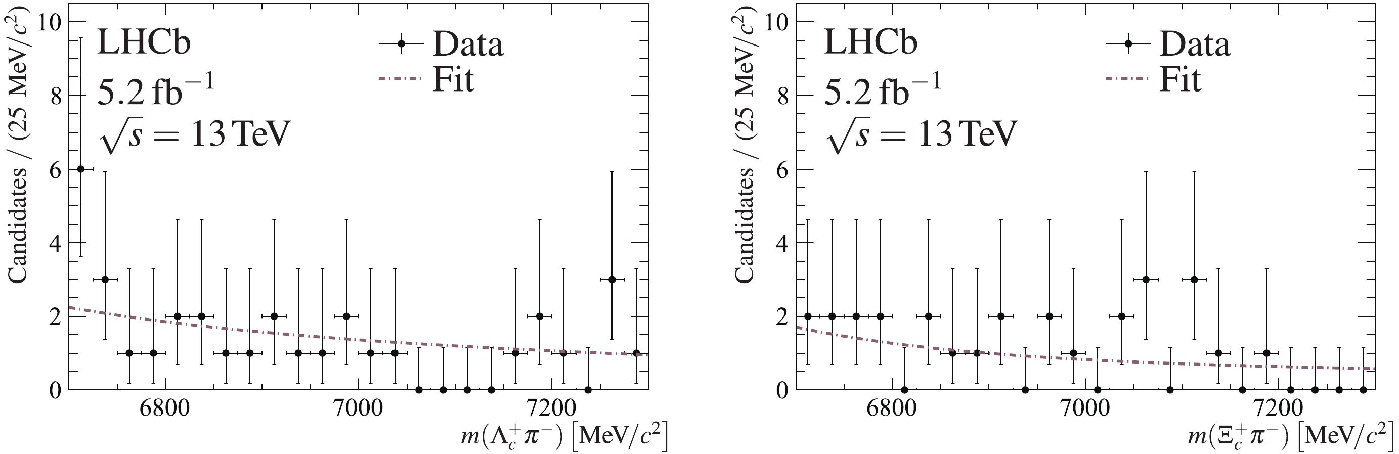
Figure 2. (color online) Invariant mass distributions of selected (left)
$ {{{{{{H_{bc}^{0}}}} {{\rightarrow }}{{{{\varLambda}^+_c}}}{{{{\pi}^-}}}}}} $ and (right)$ {{{{{{H_{bc}^{0}}}} {{\rightarrow }}{{{{\varXi}^+_c}}}{{{{\pi}^-}}}}}} $ candidates (black points), together with results of the background only fit (brown dashed line).The
$ {{{{\varLambda}^+_c}}}{{{{\pi}^-}}} $ and$ {{{{\varXi}^+_c}}}{{{{\pi}^-}}} $ invariant mass distributions of the selected$ {{{{{{{{\varLambda}^0_b}}}{{\rightarrow }}{{{{\varLambda}^+_c}}}({{\rightarrow }}\ p {{{K^-}}} {{{{\pi}^+}}}){{{{\pi}^-}}}}}}} $ and$ {{{{{{{{\varXi}_{b}^{0}}}}{{\rightarrow }} {{{{\varXi}^+_c}}}({{\rightarrow }} $ $ \ p {{{K^-}}} {{{{\pi}^+}}}){{{{\pi}^-}}}}}}} $ candidates are shown in Fig. 3. The yields are obtained from unbinned maximum-likelihood fits to the invariant mass distributions, using the fit model described above. The yields are determined to be$ 191\,000\pm 500 $ and$ 5\,490\pm 80 $ for$ {{{{{{{{\varLambda}^0_b}}}{{\rightarrow }}{{{{\varLambda}^+_c}}}({{\rightarrow }}\ p {{{K^-}}} {{{{\pi}^+}}}){{{{\pi}^-}}}}}}} $ and$ {{{{{{{{\varXi}_{b}^{0}}}}{{\rightarrow }}{{{{\varXi}^+_c}}}({{\rightarrow }}\ p {{{K^-}}} {{{{\pi}^+}}}){{{{\pi}^-}}}}}}} $ , respectively.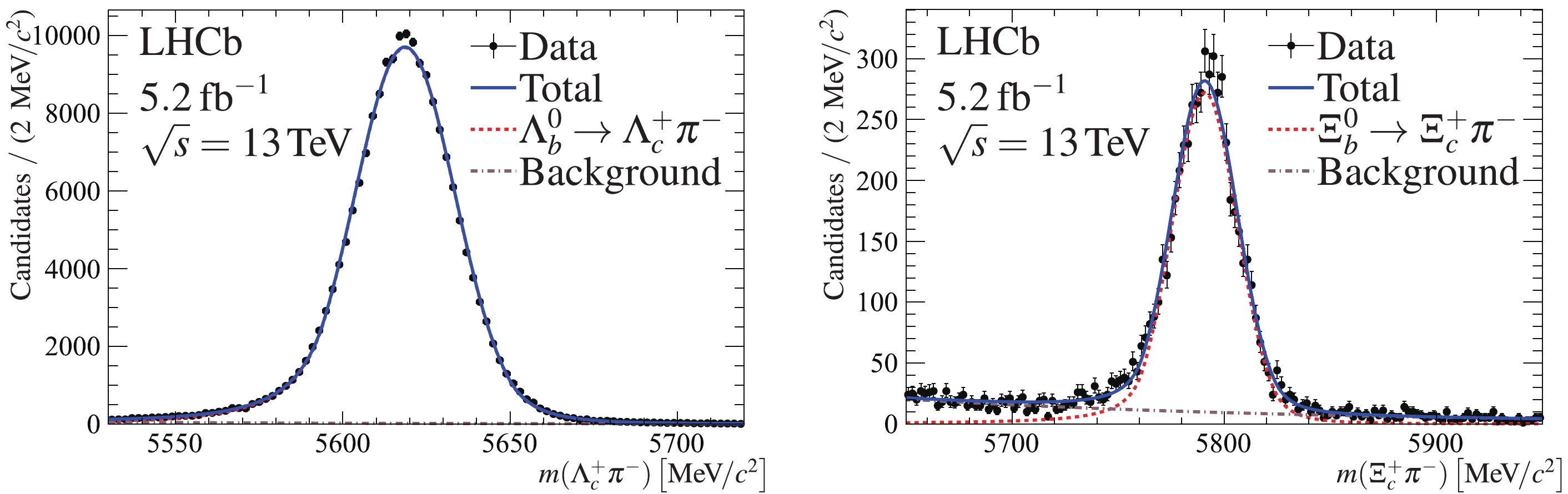
Figure 3. (color online) Invariant mass distributions of (left)
$ {{{{{{{\varLambda}^0_b}}}{{\rightarrow }}{{{{\varLambda}^+_c}}}({{\rightarrow }}\ p {{{K^-}}} {{{{\pi}^+}}}){{{{\pi}^-}}}}}} $ and (right)$ {{{{{{{\varXi}_{b}^{0}}}}{{\rightarrow }}{{{{\varXi}^+_c}}}({{\rightarrow }}\ p {{{K^-}}} {{{{\pi}^+}}}){{{{\pi}^-}}}}}} $ candidates with the fit results overlaid (blue solid line). The black points represent the data, the red dashed line represents the signal contribution, and the gray dashed line represents the combinatorial background. -
The ratio
$ \cal{R} $ of the$ {{{H_{bc}^{0}}}} $ baryon production cross-section multiplied by the branching fraction of the$ {{{{{{H_{bc}^{0}}}} {{\rightarrow }}{{{{\varLambda}^+_c}}}{{{{\pi}^-}}}}}} ({{{{{{H_{bc}^{0}}}} {{\rightarrow }}{{{{\varXi}^+_c}}}{{{{\pi}^-}}}}}})$ decay relative to that of the$ {{{{\varLambda}^0_b}}} $ ($ {{{{\varXi}_{b}^{0}}}} $ ) baryon can be written as$ \begin{aligned}[b] {\cal{R}}({{{{\varLambda}^+_c}}}{{{{\pi}^-}}})\equiv &\frac{\sigma(pp {{\rightarrow }} {{{H_{bc}^{0}}}} X)\ {{{{\mathcal{B}}}}}\left( {{{{{{H_{bc}^{0}}}}{{\rightarrow }}{{{{\varLambda}^+_c}}}({{\rightarrow }}\ p {{{K^-}}} {{{{\pi}^+}}}){{{{\pi}^-}}}}}} \right)}{\sigma(pp {{\rightarrow }} {{{{\varLambda}^0_b}}} X)\ {{{{\mathcal{B}}}}}\left( {{{{{{{\varLambda}^0_b}}}{{\rightarrow }}{{{{\varLambda}^+_c}}}({{\rightarrow }}\ p {{{K^-}}} {{{{\pi}^+}}}){{{{\pi}^-}}}}}} \right)}\\ =& \frac{N({{{{{{H_{bc}^{0}}}} {{\rightarrow }}{{{{\varLambda}^+_c}}}{{{{\pi}^-}}}}}})}{N({{{{{{{\varLambda}^0_b}}}{{\rightarrow }}{{{{\varLambda}^+_c}}}{{{{\pi}^-}}}}}})}\cdot \frac{\varepsilon({{{{\varLambda}^0_b}}})}{\varepsilon({{{H_{bc}^{0}}}})}, \end{aligned} $

(1) $ \begin{aligned}[b] {\cal{R}}({{{{\varXi}^+_c}}}{{{{\pi}^-}}})\equiv &\frac{\sigma(pp {{\rightarrow }} {{{H_{bc}^{0}}}} X)\ {{{{\mathcal{B}}}}}\left( {{{{{{H_{bc}^{0}}}}{{\rightarrow }}{{{{\varXi}^+_c}}}({{\rightarrow }}\ p {{{K^-}}} {{{{\pi}^+}}}){{{{\pi}^-}}}}}} \right)}{\sigma(pp {{\rightarrow }} {{{{\varXi}_{b}^{0}}}} X)\ {{{{\mathcal{B}}}}}\left( {{{{{{{\varXi}_{b}^{0}}}}{{\rightarrow }}{{{{\varXi}^+_c}}}({{\rightarrow }}\ p {{{K^-}}} {{{{\pi}^+}}}){{{{\pi}^-}}}}}} \right)} \\ = & \frac{N({{{{{{H_{bc}^{0}}}} {{\rightarrow }}{{{{\varXi}^+_c}}}{{{{\pi}^-}}}}}})}{N({{{{{{{\varXi}_{b}^{0}}}}{{\rightarrow }}{{{{\varXi}^+_c}}}{{{{\pi}^-}}}}}})}\cdot \frac{\varepsilon({{{{\varXi}_{b}^{0}}}})}{\varepsilon({{{H_{bc}^{0}}}})}, \end{aligned} $

(2) where N and
$ \varepsilon $ are the signal yield and the efficiency for the corresponding decay modes, respectively. The efficiency accounts for the geometrical acceptance, trigger, reconstruction, and event selection. The$ \cal{R} $ is determined in the fiducial region$ 2<y<4.5 $ and$ 2<{{p_{\rm{T}}}}<20 \;{\rm{MeV}}/{c} $ .Efficiencies are determined from the simulated samples. The
$ {{p_{\rm{T}}}} $ distributions of$ {{{{\varLambda}^0_b}}} $ and$ {{{{\varXi}_{b}^{0}}}} $ baryons are not well modeled in simulation. To improve the description, a gradient boosted weighting method [57] is used to apply a kinematic correction on the$ {{p_{\rm{T}}}} $ distributions of the$ {{{{\varLambda}^0_b}}} $ and$ {{{{\varXi}_{b}^{0}}}} $ decay products of the simulated control samples. With this correction, a good agreement on the$ {{{{\varLambda}^0_b}}} $ and$ {{{{\varXi}_{b}^{0}}}} $ $ {{p_{\rm{T}}}} $ distribution is seen between the data and simulation. The track detection and particle identification efficiencies are calibrated with the data [58-60]. The imperfect modeling of input variables used in the BDT training can bias the efficiency estimation. To suppress such effects, ratios between the BDT response distribution of the background-subtracted data sample and that of the simulated sample are calculated using the control channel. The background subtraction is performed using the$ {sPlot} $ method [61] with$ m({{{{\varLambda}^+_c}}}{{{{\pi}^-}}}) $ and$ m({{{{\varXi}^+_c}}}{{{{\pi}^-}}}) $ as discriminating variables. These ratios are applied as correction weights to the simulated samples for all reconstructed decay modes.The total efficiency ratio
$ \varepsilon({{{{\varLambda}^0_b}}})/\varepsilon({{{H_{bc}^{0}}}}) $ is determined to be$ 3.18\pm0.05 $ , and$ \varepsilon({{{{\varXi}_{b}^{0}}}})/\varepsilon({{{H_{bc}^{0}}}}) $ is calculated to be$ 3.00\pm0.02 $ for$ m({{{H_{bc}^{0}}}}) = 6900 \;{\rm{MeV}}/{c^2} $ and$ \tau({{{H_{bc}^{0}}}}) = 0.4\;{\rm{ps}} $ . The efficiency is larger for the control mode, mainly due to the longer lifetime of the$ {{{{\varLambda}^0_b}}} $ and$ {{{{\varXi}_{b}^{0}}}} $ baryons. The efficiency depends on the mass and lifetime hypotheses of the$ {{{H_{bc}^{0}}}} $ state, and is evaluated from simulation. The kinematic properties of the fully simulated samples are weighted to match those of the generator-level sample to calculate the efficiency for different$ {{{H_{bc}^{0}}}} $ mass and lifetime assumptions. -
Various sources of systematic uncertainties on
$ {\cal{R}} $ are estimated and combined in quadrature. The effect of imperfect description of the mass distributions on the yield estimates is studied using alternative signal and background models. For the signal model, the Hypatia [62] function is used instead of the nominal double-sided Crystal Ball function. For the background model of the control modes, the nominal double-exponential function is replaced by a first-order polynomial function. As the background model for the$ {{{H_{bc}^{0}}}} $ decay modes is interpolated from the sidebands, its uncertainty is evaluated by both replacing the nominal function with an exponential function and varying the sideband regions. The largest deviation with respect to the nominal result is taken as the corresponding uncertainty. In total, the associated systematic uncertainty is estimated to be 0.1% and 0.9% for$ {{{{{{{H_{bc}^{0}}}} {{\rightarrow }}{{{{\varLambda}^+_c}}}{{{{\pi}^-}}}}}}} $ and$ {{{{{{{H_{bc}^{0}}}} {{\rightarrow }}{{{{\varXi}^+_c}}}{{{{\pi}^-}}}}}}} $ decays, respectively.In the
$ {\cal{R}} $ ratios, systematic uncertainties arising from the track detection efficiency largely cancel, and the uncertainty due to limited size of simulation samples is determined to be 1.6% (0.7%) on$ {\cal{R}} ({{{{\varLambda}^+_c}}}{{{{\pi}^-}}}) $ ($ {\cal{R}} ({{{{\varXi}^+_c}}}{{{{\pi}^-}}}) $ ). The particle identification efficiency is determined in bins of particle momentum, pseudorapidity, and track multiplicity using control channels in the data [60]. As the particle identification variables have large dependencies on the momentum of the final-state particles, there are sizeable differences in these efficiencies between the control and signal channels, which do not cancel in the ratio measurement. Systematic effects arising from the choice of binning scheme are evaluated by varying the bin sizes and reevaluating the efficiency. The largest deviations from the nominal result, 1.7% and 2.1%, are assigned as the systematic uncertainty for the$ {{{{{{{H_{bc}^{0}}}} {{\rightarrow }}{{{{\varLambda}^+_c}}}{{{{\pi}^-}}}}}}} $ and$ {{{{{{{H_{bc}^{0}}}} {{\rightarrow }}{{{{\varXi}^+_c}}}{{{{\pi}^-}}}}}}} $ decays, respectively.The
$ {{{{\varLambda}^+_c}}} $ ($ {{{{\varXi}^+_c}}} $ ) mass resolution shows a difference between data and simulation, which affects the selection efficiency. It results in a 0.2% systematic uncertainty contribution for the$ {{{{{{{H_{bc}^{0}}}} {{\rightarrow }}{{{{\varXi}^+_c}}}{{{{\pi}^-}}}}}}} $ decay, while the contribution for the$ {{{{{{{H_{bc}^{0}}}} {{\rightarrow }}{{{{\varLambda}^+_c}}}{{{{\pi}^-}}}}}}} $ decay is below 0.1%. This systematic uncertainty is negligible compared to other sources.The imperfect simulation of the signal and control modes are considered by applying corrections to the BDT response and kinematic properties of the simulated control mode samples. To assess the systematic uncertainty in these corrections, the correcting weights are varied within their uncertainties. The largest deviation from the nominal result is taken as the systematic uncertainty. Combining the uncertainties from the BDT response correction and the kinematic modeling of the simulated control samples gives an uncertainty of 1.6% for the
$ {{{{{{{H_{bc}^{0}}}} {{\rightarrow }}{{{{\varLambda}^+_c}}}{{{{\pi}^-}}}}}}} $ channel, and 3.0% for the$ {{{{{{{H_{bc}^{0}}}} {{\rightarrow }}{{{{\varXi}^+_c}}}{{{{\pi}^-}}}}}}} $ channel. The analysis relies on the$ {{{{\varXi}_{bc}^{0}}}} $ $ {{p_{\rm{T}}}} $ model implemented in simulation. No systematic uncertainty is assigned to this model.The algorithm used to compute the
$ {\chi^2_{\rm{IP}}} $ was updated during data collection, which causes a mismatch between data and simulation and introduces systematic effects in the efficiency estimation. The corresponding uncertainty was found to be 5% in the previous$ {{{{\varXi}_{bc}^{0}}}} $ search [29]. Checks by varying the$ {\chi^2_{\rm{IP}}} $ -related requirements show that the uncertainty well covers the change of result. Therefore, a 5% systematic uncertainty is assigned.The systematic uncertainties are summarized in Table 1. The total systematic uncertainty is 5.7% for
$ {{{{{{{H_{bc}^{0}}}} {{\rightarrow }}{{{{\varLambda}^+_c}}}{{{{\pi}^-}}}}}}} $ and 6.3% for$ {{{{{{{H_{bc}^{0}}}} {{\rightarrow }}{{{{\varXi}^+_c}}}{{{{\pi}^-}}}}}}} $ , for a$ {{{H_{bc}^{0}}}} $ mass of 6900$ \;{\rm{MeV}}/{c^2} $ and lifetime of 0.4$ \;{\rm{ps}} $ . These values of systematic uncertainties are also used for other assumed lifetime and mass hypotheses.${{{{{{H_{bc}^{0}}}} {{\rightarrow }}{{{{\varLambda}^+_c}}}{{{{\pi}^-}}}}}}$ 

${{{{{{H_{bc}^{0}}}} {{\rightarrow }}{{{{\varXi}^+_c}}}{{{{\pi}^-}}}}}}$ 

Fit model 0.1% 0.9% Size of simulated samples 1.6% 0.7% Particle identification efficiency 1.7% 2.1% Mass resolution <0.1% 0.2% Simulation model 1.6% 3.0% $ {\chi^2_{\rm{IP}}} $ simulation

5.0% 5.0% Total 5.7% 6.3% Table 1. Sources of systematic uncertainty obtained for an
$ {{{H_{bc}^{0}}}} $ mass of 6900$ \;{\rm{MeV}}/{c^2} $ and lifetime of 0.4$ \;{\rm{ps}} $ . The total is the quadratic sum of the individual systematic uncertainties. -
No evidence for a
$ {{{{\varOmega}_{bc}^{0}}}} $ or a$ {{{{\varXi}_{bc}^{0}}}} $ baryon is observed in the inspected mass range. Upper limits are set at 95% confidence level on the ratios$ {\cal{R}}({{{{\varLambda}^+_c}}}{{{{\pi}^-}}}) $ and$ {\cal{R}}({{{{\varXi}^+_c}}}{{{{\pi}^-}}}) $ under different mass and lifetime hypotheses for the$ {{{{\varOmega}_{bc}^{0}}}} $ and$ {{{{\varXi}_{bc}^{0}}}} $ baryons, using the asymptotic$ {{\rm{CL }}_{s}} $ method implemented in the$ {{\mathsf{ROOSTATS}}} $ framework [63, 64] considering the systematic uncertainties. The assumed masses of the$ {{{{\varOmega}_{bc}^{0}}}} $ and$ {{{{\varXi}_{bc}^{0}}}} $ baryons are varied from 6700 to 7300$ \;{\rm{MeV}}/{c^2} $ with a step size of 4$ \;{\rm{MeV}}/{c^2} $ , and the lifetime values of 0.2$ \;{\rm{ps}} $ , 0.3$ \;{\rm{ps}} $ , and 0.4$ \;{\rm{ps}} $ are considered. The calculated upper limits are shown in Fig. 4, as a function of the$ {{{H_{bc}^{0}}}} $ mass. These results are obtained for the sum of the$ {{{{\varOmega}_{bc}^{0}}}} $ and$ {{{{\varXi}_{bc}^{0}}}} $ production and as such hold for the two individually.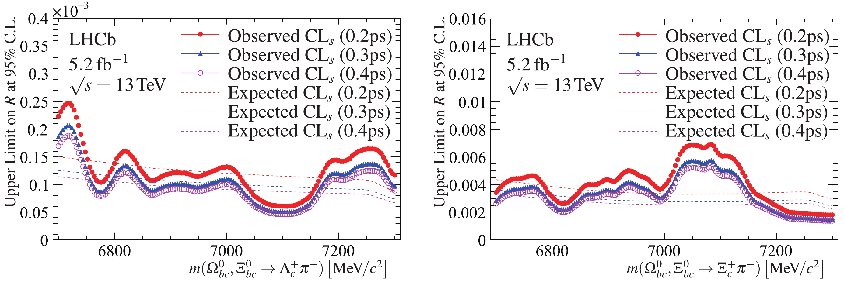
Figure 4. (color online) Upper limits (dotted lines) on the ratio of production cross-section for
$ {{{{\varOmega}_{bc}^{0}}}} $ and$ {{{{\varXi}_{bc}^{0}}}} $ via decays to (left)$ {{{{\varLambda}^+_c}}}{{{{\pi}^-}}} $ and (right)$ {{{{\varXi}^+_c}}}{{{{\pi}^-}}} $ to that of control channels$ {{{{{{{\varLambda}^0_b}}}{{\rightarrow }}{{{{\varLambda}^+_c}}}{{{{\pi}^-}}}}}} $ and$ {{{{{{{\varXi}_{b}^{0}}}}{{\rightarrow }}{{{{\varXi}^+_c}}}{{{{\pi}^-}}}}}} $ . The dotted (dashed) colored lines represent the observed (expected) upper limits. The assumed lifetime hypotheses for the$ {{{{\varOmega}_{bc}^{0}}}} ({{{{\varXi}_{bc}^{0}}}}) $ are 0.2 ps (red filled circles), 0.3 ps (blue triangles), and 0.4 ps (magenta open circles). -
The first search for the doubly heavy baryon
$ {{{{\varOmega}_{bc}^{0}}}} $ and a new search for the$ {{{{\varXi}_{bc}^{0}}}} $ baryon in the mass range from 6700 to 7300$ \;{\rm{MeV}}/{c^2} $ are presented, using$ pp $ collision data collected at a centre-of-mass energy$ {{\sqrt{s}}} = 13 \;{\rm{TeV}} $ with the$ {\rm{LHCb}} $ experiment. The data set corresponds to an integrated luminosity of 5.2$ \;{\rm{f}}{{\rm{b}}^{ - 1}} $ . The$ {{{{\varOmega}_{bc}^{0}}}} $ ($ {{{{\varXi}_{bc}^{0}}}} $ ) baryon is reconstructed in the$ {{{{\varLambda}^+_c}}}{{{{\pi}^-}}} $ and$ {{{{\varXi}^+_c}}}{{{{\pi}^-}}} $ decay modes. No evidence of a signal is found. Upper limits at 95% confidence level on the ratio of the$ {{{{\varOmega}_{bc}^{0}}}} $ ($ {{{{\varXi}_{bc}^{0}}}} $ ) production cross-section times its branching fraction relative to that of the$ {{{{\varLambda}^0_b}}} $ ($ {{{{\varXi}_{b}^{0}}}} $ ) baryon are calculated in the rapidity range$ 2.0 < y < 4.5 $ and transverse momentum range$ 2<{{p_{\rm{T}}}} < 20 \;{\rm{MeV}}/{c} $ under different$ {{{{\varOmega}_{bc}^{0}}}} $ ($ {{{{\varXi}_{bc}^{0}}}} $ ) mass and lifetime hypotheses. The upper limits range from$ 0.5\times10^{-4} $ to$ 2.5\times10^{-4} $ for the$ {{{{{{{{\varOmega}_{bc}^{0}}}}{{\rightarrow }}{{{{\varLambda}^+_c}}}{{{{\pi}^-}}}}}} ({{{{{{{\varXi}_{bc}^{0}}}}{{\rightarrow }}{{{{\varLambda}^+_c}}}{{{{\pi}^-}}}}}})} $ decay, and from$ 1.4\times10^{-3} $ to$ 6.9\times10^{-3} $ for the$ {{{{{{{{\varOmega}_{bc}^{0}}}}{{\rightarrow }}{{{{\varXi}^+_c}}}{{{{\pi}^-}}}}}} ({{{{{{{\varXi}_{bc}^{0}}}}{{\rightarrow }}{{{{\varXi}^+_c}}}{{{{\pi}^-}}}}}})} $ decay, for the considered lifetime and mass hypotheses. These results constitute the first limit on the production of the$ {{{{\varOmega}_{bc}^{0}}}} $ baryon. Further measurements will be possible with the larger data samples expected at the upgraded$ {\rm{LHCb}} $ experiments [65] and with additional decay modes. -
We express our gratitude to our colleagues in the CERN accelerator departments for the excellent performance of the LHC.
Search for the doubly heavy baryons ${\boldsymbol \varOmega_{\boldsymbol{bc}}^{\bf 0}} $ and $ {\boldsymbol\varXi_{\boldsymbol{bc}}^{\bf 0} }$ decaying to ${ \boldsymbol \varLambda_c^+\pi^- }$ and $ {\boldsymbol\varXi_c^+\pi^- }$
- Received Date: 2021-05-27
- Available Online: 2021-09-15
Abstract: The first search for the doubly heavy


 DownLoad: