Isgur-Wise function in B_c decays to charmonium with the Bethe-Salpeter method

Under the heavy quark effective theory (HQET), a semileptonic decay process can be related to a rotation of the heavy quark flavor or spin [1, 2]. In the limit $m_Q\to\infty$ (Q denotes a heavy quark or anti-quark), this rotation is a symmetry transformation. The form factors depend only on the Lorentz boost $\gamma = v\cdot v'$ which connects the rest frames of the initial state and the final state. The transition can be described by a dimensionless function $\xi(v\cdot v')$. Heavy-quark symmetry reduces the weak-decay form factors of heavy hadrons to this universal function. These relations were derived by Isgur and Wise firstly [3, 4], the so-called Isgur-Wise function (IWF).

The HQET vastly simplifies these calculations; thus, it plays a crucial role in extracting the values of $|V_{cb}|$ and $|V_{ub}|$. For example, the differential semileptonic decay rate for $B\to D$ in the heavy-quark limit can be model-independently described by [2]

The decay rate depends on only two quantities, $|V_{cb}|$ and $\xi(\omega)$. If the differential semileptonic decay rate is measured by experiments, one can obtain the value of $|V_{cb}|\xi(\omega)$. Exploiting the normalization of the Isgur-Wise function $\xi(1) = 1$, the value of $|V_{cb}|$ can be extracted. Conversely, exploiting the given value of $|V_{cb}|$, the differential semileptonic decay rate can be obtained by calculating the Isgur-Wise function. However, the Isgur-Wise function cannot be calculated by perturbation theory in principle and can only be obtained by various phenomenological models. Obviously, the latter method is model-dependent. Then, substantial effort has been directed toward studying the Isgur-Wise function and its applications in different frameworks [5-16]. In a phenomenological model, the Isgur-Wise function usually corresponds to the overlapping integral of the wave functions.

However, the leading order result is not sufficiently accurate because of the heavy quark approximation. The symmetry-breaking corrections are needed when the study becomes more precise, since the masses of the heavy quarks or anti-quarks are not actually infinite. In addition, the radiation correction cannot be ignored. The HQET provides a systematic framework to analyze these corrections. For example, Luke analyzed the $1/m_Q$ corrections for a more complicated case of weak decay form factors [17]. Falk et al. analyzed the structure of $1/m^2_Q$ corrections for weak decay form factors of both mesons and baryons and calculated the leading QCD radiative corrections [18, 19]. Other efforts of complements are too numerous to be listed here [20-22].

The flavor-spin symmetry can be used for weak decays involving not only ground hardons, but also orbitally and radially excited states containing one heavy (anti-) quark. For example, Isgur and Wise exploited the flavor-spin symmetry to obtain model-independent predictions in weak decays from the pseudoscalar meson of a heavy quark $Q_i$ to P wave excited states of another heavy quark $Q_j$ in terms of two Isgur-Wise functions [23]; other studies have also reported interesting results [24-27]. The HQET is not adopted here; therefore, we do not describe it in detail to avoid confusion.

When systems contain two or more heavy degrees of freedom, the validity of HQET doubtful, but they are still best described in the nonrelativistic QCD (NRQCD). However, some studies have explored the application of the heavy quark symmetry to describe the weak decays of hadrons containing two heavy quarks. Sanchis-Lozano estimated the flavor symmetry loss, while the spin symmetry holds for the double-heavy meson [28]. A baryon containing two heavy quarks constitutes a bosonic diquark whose mass can be regarded as infinite; therefore, HQET still holds true for the diquark-light quark system. However, HQET is not suitable for dealing with the diquark subsystem. Ebert et al. exploited the relativistic quark model to obtain the diquark wave functions; then, the transition amplitudes of heavy diquarks bb and bc going respectively to bc and cc can be expressed through the overlap integrals of corresponding diquark wave functions [29]. Pathak et al. treated the $B_c$ meson as a typical heavy-light meson like B or D within a QCD potential model, and the semileptonic decay rates of $B_c$ meson into $\eta_c$, $J/\psi$ are exploited [30]. Das et al. computed the slopes and curvatures of the form factors of semileptonic decays of heavy-light mesons including $B_c$ [31]. The error of the result for $B_c$ is very large. Wang et al. obtained form factors for $B_c$ into the S-wave and P-wave charmonium using three universal Isgur-Wise functions [32]. Nearly all of these studies adopt the formulas in HQET directly, but the usefulness of the heavy quark symmetry to describe double heavy hadrons has seldom been reported.

The aim of this paper is to investigate the heavy quark symmetry in double-heavy mesons from a phenomenological aspect free of the heavy quark limit. The heavy quark symmetry, if it holds roughly, must be reflected in the results obtained by a suitable phenomenological model without the employment of the heavy quark limit. The instantaneous Bethe-Salpeter (BS) equation is quite effective for dealing with double-heavy mesons. This method has a comparatively solid foundation because both the BS equation and the Mandelstam formula are established based on relativistic quantum field theory. Meanwhile, the instantaneous approximation is reasonable because the quark and antiquark in double-heavy mesons are both heavy. This method gives an analytical expression, so the symmetry can be found intuitively, although the accuracy may not be as good as in Lattice QCD. We choose the semileptonic $B_c$ decays to charmonium, and the final mesons involve the orbitally and radially excited states. It is concluded that the flavor symmetry breaks, while the spin symmetry holds for the double-heavy meson, as Sanchis-Lozano estimated [28]. The HQET is applicable to these decays in this paper from a phenomenological aspect because the spectator charm quark is not involved in the hard scattering over a short time scale, on the order of $1/m_W$ [32]. However, the form factors parameterized by a single Isgur-Wise function deviate seriously from the full ones, especially when excited states are involved. The relativistic corrections require the introduction of more non-perturbative universal functions, similar to the Isgur-Wise function.

Previous studies of the IWF with the BS equation have been performed. Kugo et al. expanded the BS equation in the order of the inverse heavy quark mass and defined the leading term in the expansion of the first form factor as the IWF [33]. El-Hady et al. pointed out that the IWF can be related to the overlap integral of normalized meson wave functions in the infinite momentum frame and that it should be possible to calculate the form factors directly without using the heavy quark limit [34]. Zoller et al. calculated the numerical IWF by multiplying quark masses with a large factor directly [35]. Chang et al. obtained two universal functions in $B_c\to h_c,\chi_{c}$ with the instantaneous BS method, but the wave functions they used are nonrelativistic [36, 37]. Recently, the instantaneous BS method has been developed to be quite covariant, and the full Salpeter equations are solved for different $J^{P(C)}$ states [38-41]. Therefore, the relativistic correction, which equates to the symmetry-breaking correction, has better been taken into account. Note that in this paper we do not use HQET, but we rather attempt to examine the validity of HQET on double heavy mesons using the instantaneous BS method from a phenomenological aspect. The heavy quark limit is also not adopted here.

This paper is organized as follows. In Sec. II, we give the relativistic wave function and Mandelstam formalism for the instantaneous BS method. In Sec. III, we extract the IWF and give the analytical results. In Sec. IV, we give the numerical results and discussions. We summarize and conclude in Sec. V, and the Salpeter equation and some wave functions are described in Appendix A.

Usually, the nonrelativistic wave function for a pseudoscalar is written as [36]

where M and P are the mass and momentum of the meson, respectively; $\vec{q}$ is the relative momentum between the quark and antiquark, and the radial wave function $f(\vec{q})$ can be obtained by solving the Schrodinger equation. However, in our method, we solve the full Salpeter equation. The form of the wave function is relativistic and should depend on the $J^{P(C)}$ quantum number of the corresponding meson. The relativistic wave function of a pesudosclar can be constructed using P, $q_{\perp}$, and $\gamma$-matrices [42]

where $q = p_1-\alpha_1 P = \alpha_2 P-p_2$ is the relative momentum between a quark (with momentum $p_1$ and mass $m_1$) and antiquark (momentum $p_2$ and mass $m_2$), $\alpha_1 = \displaystyle\frac{m_1}{m_1+m_2}$, $\alpha_2 = \displaystyle\frac{m_2}{m_1+m_2}$; $q_{\perp} = q-\displaystyle\frac{P\cdot q}{M^2}P$, in the rest frame of the meson, $q_{\perp} = (0,\vec{q})$.

The quantum numbers of all items in Eq. (3) are $0^-$. This wave function is a general relativistic form for a pseudoscalar with the instantaneous approximation. If we drop the ${\cal{O}}(\frac{{\not q}_{\perp}}{M})$ items and ignore the difference between $f_1$ and $f_2$, Eq. (3) would be reduced to the Schrodinger wave function, Eq. (2).

The procedure to solve the full Salpeter equation is given in Appendix A. The last two equations in Eq. (A9) are constraint equations; therefore, only two wave functions in Eq. (3) are independent. We retain $f_1$ and $f_2$ and derive the normalization condition as

where the quark energy $\omega_i = \sqrt{m^2_i-q_{\perp}^2} = \sqrt{m^2_i+\vec{q}^{\:2}}$ ($i = 1,2$). The projection operators are defined as

and the positive energy wave function is

where

In this paper, in addition to the $0^-$ state, we also need to construct the wave functions for the $1^{--}$ ($J/\psi$), $1^{+-}$ ($h_c$), $0^{++}$ ($\chi_{c0}$), $1^{++}$ ($\chi_{c1}$), and $2^{++}$ ($\chi_{c2}$) states. We show the $2^{++}$ state wave function in Appendix A, and the others can be found in [43].

The transition amplitude element for $B_c^+\to (c\bar c)\ell^+\nu_{\ell}$ shown in Fig. 1 reads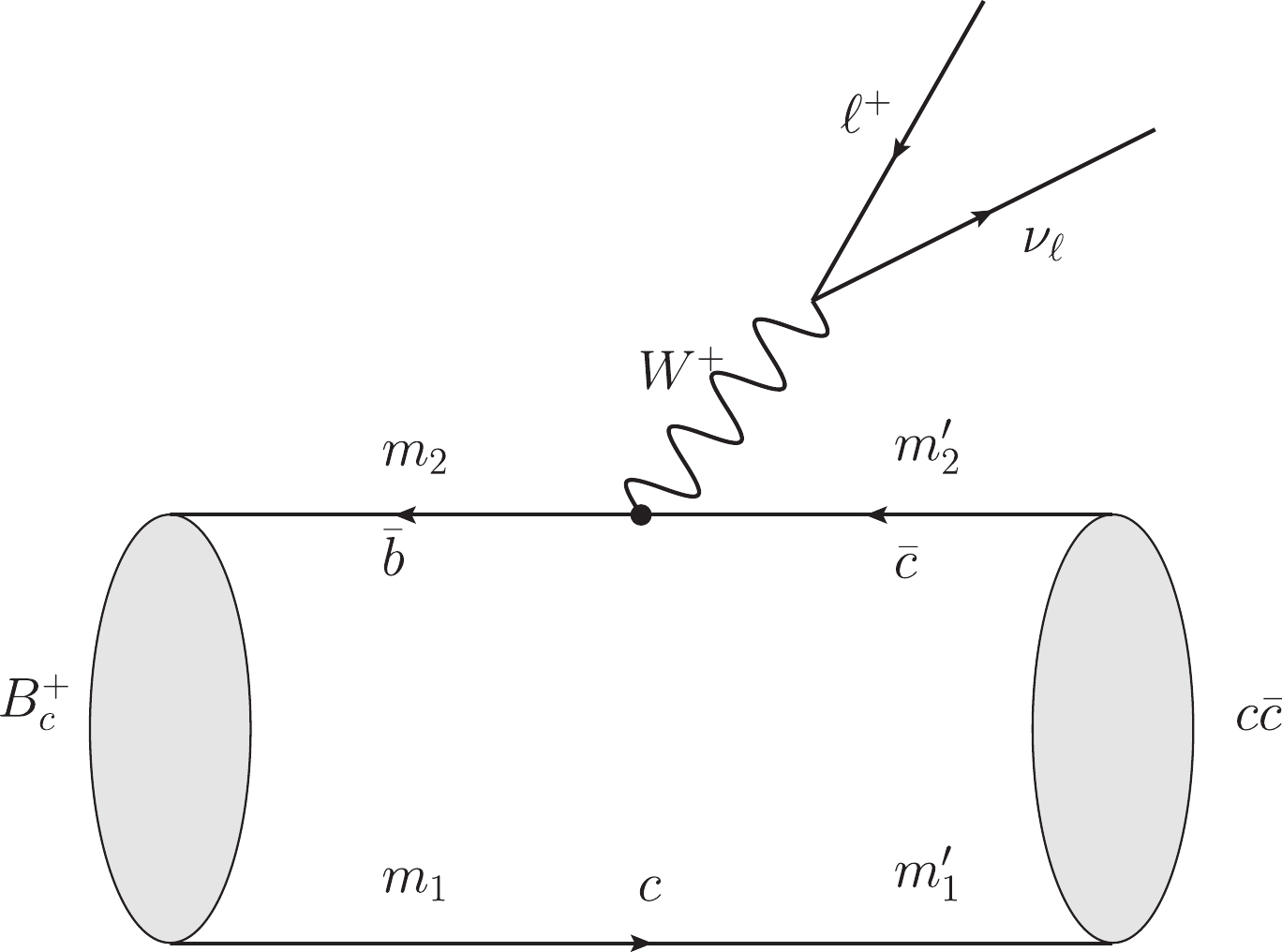

Figure 1.  Feynman diagram corresponding to the semileptonic decays $B_c^+\to (c\bar c)\ell^+\nu_{\ell}$.

where $(c\bar c)$ denotes charmonium and $J_{\mu}\equiv V_{\mu}-A_{\mu}$ is the charged current responsible for this decay. The hadronic part can be calculated using the overlapping integral over the initial and final wave functions, which we call the Mandelstam formalism. The wave function should be solved using the full relativistic BS equation, but this is difficult. Instead, we solve the instantaneous one, namely, the full Salpeter equation. The hadronic transition element should be approximated as [44]

where $\varphi_P^{++}$ denotes the positive energy wave function of the initial state and $\overline\varphi_{P_f}^{++}\equiv\gamma^0(\varphi_{P_f}^{++})^{\dagger}\gamma^0$ is that for the final state; $\vec q\:'$ is the relative momentum between a quark (with mass $m'_1$) and antiquark (mass $m'_2$) in the final state, and $\vec q = \vec q\:'+\displaystyle\frac{m'_1}{m'_1+m'_2} \vec P_f$. In this paper, we drop $\varphi^{+-},\varphi^{-+},\varphi^{--}$ and keep only the positive energy component $\varphi^{++}$, as those contributions are much smaller than 1% in the $B_c \to (c\bar c)$ transition [45]. The integral argument $\vec q\:'$ in Eq. (9) is convenient for the P-wave final state [37].

For $B_c^+\to P\ell^+\nu_{\ell}$ (here, P denotes $\eta_c$ or $\chi_{c0}$), the hadronic matrix element can be factorized as

where $S_{+}$ and $S_{-}$ are the form factors. For $B_c^+\to V\ell^+\nu_{\ell}$ (here, V denotes $J/\psi$, $h_c$, or $\chi_{c1}$),

where $\epsilon^{\mu}$ is the polarization vector of the final vector meson; $t_1$, $t_2$, $t_3$, and $t_4$ are the form factors. For $B_c^+\to T\ell^+\nu_{\ell}$ (here, T denotes $\chi_{c2}$),

where $\epsilon_{\alpha\beta}$ is the polarization tensor of the final tensor meson; $t_1$, $t_2$, $t_3$, and $t_4$ are the form factors. In this paper, we focus only on the form factors, but not the decay widths.

Because the binding energy is on the order of $\Lambda_{\rm QCD}$, which is smaller than the constituent quark mass in $B_c$ and charmonium, the approximation

is employed. In the numerical calculation, the large $|\vec q|$ contribution will be suppressed by the wave function $f_i(\vec q)$. After performing this approximation and the trace on the matrix element Eq. (9), all the form factors depend only on the overlapping integrals of the wave functions for the initial state and the final state. For instance, one type of overlapping integral is

where $f_i$ denotes the wave function of the initial state and $f'_i$ denotes the wave function of the final state. Two wave functions from the same meson are very similar numerically, i.e., $f_1\approx f_2$ and $f'_1\approx f'_2$. Therefore, the four overlapping integrals in Eq. (14) are approximately equal, and for convenience, they are replaced by their average, which is denoted as

where C is the normalization coefficient; $v,v'$ are the four dimensional velocities of the initial state and final state, respectively, and $\overline{ff'} = \displaystyle\frac{f_1f'_1+f_1f'_2+f_2f'_1+f_2f'_2}{4}$. There are other overlapping integrals with the relative momentum $\vec q\:'$ being inserted. It is immediately clear that they are the relativistic ($1/m_Q$) corrections to the leading order form factors, which are parameterized by a single function $\xi_{00}$. They are denoted as $\xi_{qx}$, where subscript q denotes the power of the relative momentum $\vec q\:'$, subscript x denotes the power of $\cos\theta$, and $\theta$ is the angle between $\vec q\:'$ and $\vec P_f$, i.e.,

and so on. When the final state is an S-wave meson, we keep the first six functions and drop the higher order ${\cal{O}}(q^4)$; when the final state is a P-wave meson, whose wave function includes a factor $\vec q$, $\xi_{00}$ disappears. Thus, we reserve the first eight functions and drop the higher order ${\cal{O}}(q^5)$. The normalization coefficients C based on the normalized formulas are shown in Table 1 for each process. Taking the process $B_c\to\eta_c$ as an example, the initial and final states are both the $0^-$ state. With the approximations $\vec q = 0$, $f_1 = f_2$, and $\omega_i = m_i$, Eq. (4) is deduced to be

final state	$\eta_c$	$J/\psi$	$h_c$	$\chi_{c0}$	$\chi_{c1}$	$\chi_{c2}$
$C$	$4\sqrt{MM'}$	$4\sqrt{MM'}$	$\frac{4M}{\sqrt{3}}$	$4M$	$4\sqrt{\frac{2}{3}}M$	$\frac{4MM'}{\sqrt{3}}$

Table 1.  Normalization coefficients of different processes.

Therefore, the normalized wave function of the $0^-$ state is $2\sqrt{M}f$, and the normalization coefficient is $4\sqrt{MM'}$ for the process $B_c\to\eta_c$. The above approximation is only used to determine the normalization coefficient, but not elsewhere.

The form factors of the semileptonic decay $B_c\to\eta_c\ell\nu_{\ell}$ can be written as

where $a_1 = E'^2-E'M+E'M'-MM' = M'(E'-M)(\omega+1)$, $a_2 = E'^2-E'M-E'M'+MM' = M'(E'-M)(\omega-1)$, $b_1 = MM'-E'M'+E'M-M'^2 = M'(M-M')(1+\omega)$, $b_2 = MM'-E'M'-E'M+M'^2 = M'(M+M')(1-\omega)$, $b_1 = \vec P_f^2-a_1$, and $b_2 = a_2-\vec P_f^2$.

where $c_1 = E'M+E'M'+MM'+M'^2$, $c_2 = E'M-E'M'- MM'+M'^2$, $d_1 = E'^2+E'M+E'M'+MM'$, $d_2 = E'^2+E'M- E'M'-MM'$, $c_1 = d_1-\vec P_f^2$, and $c_2 = d_2-\vec P_f^2$.

The function $\xi_{00}$ is just the Isgur-Wise function appearing in HQET for $0^-\to 0^-$ decays. Because the form factors of this process will degenerate into those under the nonrelativistic limit if only the function $\xi_{00}$ is considered [2],

Eq. (18) and Eq. (19) clearly show that the other functions $\xi_{qx}\; (q\neq 0)$ are the relativistic corrections ($1/m_i$ corrections) to the leading order form factors, which are parameterized by a single IWF $\xi_{00}$, where i denotes a quark or anti-quark in the initial and the final mesons. The number of $\vec q\:'$ contained in the function $\xi_{qx}$ (subscript q) corresponds to the order of the correction. Note that there should have been another type of overlapping integral with the relative momentum $\vec q$ in the initial state. For example,

where $\beta$ is the angle between $\vec q$ and $\vec P_f$. Because of the relation $\vec q = \vec q\:'+\alpha \vec P_f, \alpha = \frac{m'_1}{m'_1+m'_2}$, this overlapping integral Eq. (21) is decomposed into $\xi_{11}+\alpha|\vec P_f\:|\xi_{00}$. Therefore, the item involving $\alpha\xi_{00}$ should be considered as a relativistic correction on the same order as $\xi_{11}$. Generally, the item involving $\alpha^n\xi_{qx}$ is the $q+n$ order relativistic correction ($1/m_i^{q+n}$ correction), which can be confirmed in Eqs. (18) and (19). The process $0^-\to 1^{--}$ is the same as in the above case. The leading order result agrees with HQET [2], i.e.,

It is natural that the leading order analytical results in this paper, Eq. (20) and Eq. (22), are entirely consistent with HQET for $0^-\to 0^-$ or $1^{--}$ processes. Because, for the leading order results, the terms involving ${\not\!\!q}$ disappear and $\omega_i = m_i$, the BS wave functions degenerate into the nonrelativistic case, i.e.,

A pseudoscalar meson and its corresponding vector have the same radial wave function $\Psi$ in the nonrelativistic limit. However, in this paper, the radial wave functions are obtained by solving the BS equation numerically, and the $\Psi$ in Eq. (23) corresponds to the normalized wave function $2\sqrt{M}f_i$, where $f_i$ are the independent components of the BS wave function, similar to $f_1$ and $f_2$ in Eq. (3). Because we do not use the heavy quark limit, the normalized radial wave functions of a pseudoscalar meson and its corresponding vector are not exactly the same numerically; see Figs. 2(b) and 2(c). Furthermore, the normalized radial wave functions of $B_c$ and $\eta_c$ differ greatly; see Figs. 2(a) and 2(b). Then, the IWF $\xi_{00}$ in this paper is not the leading order result in HQET, but the corrected IWF in HQET, which contains the relativistic corrections ($1/m_Q$ corrections). However, our results in section 4 show that the form factors parameterized by this corrected IWF $\xi_{00}$ still deviate seriously from the full ones, especially involving the excited states, even if the relativistic ($1/m_Q$ corrections) correction to $\xi_{00}$ has been taken into account. It is therefore necessary to introduce more non-perturbative universal functions $\xi_{qx} (q\neq 0)$ to obtain more accurate form factors. We call these the high order correction functions below.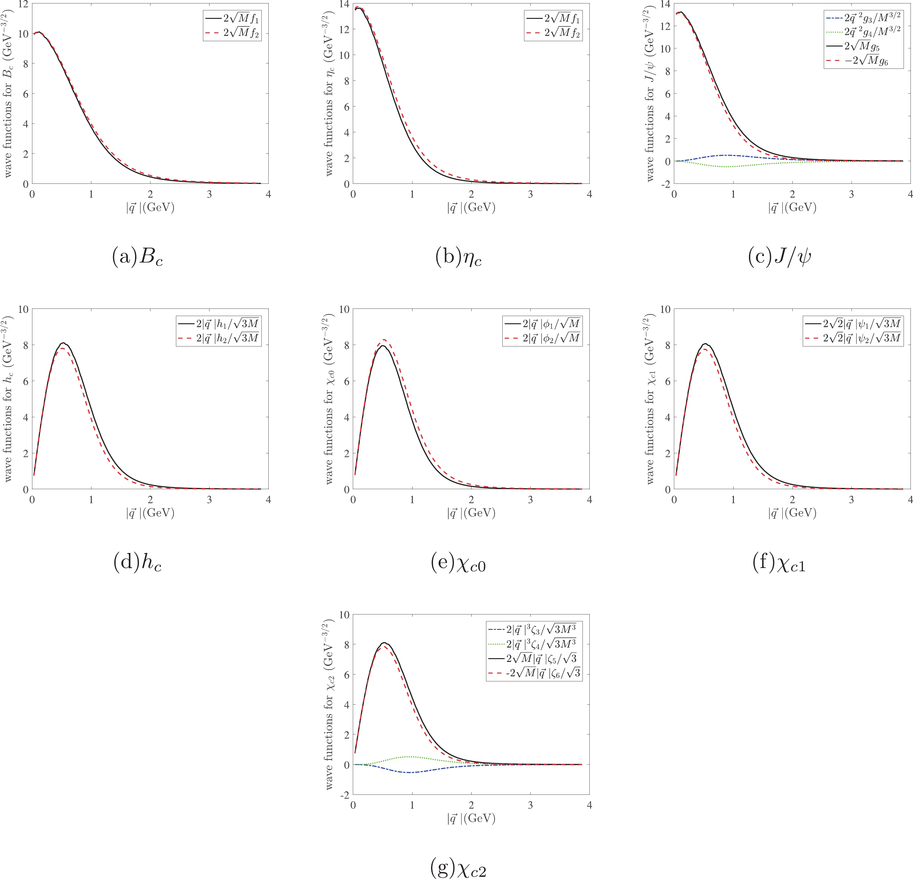

Figure 2.  (color online) Normalized radial wave functions of $B_c$ and charmonium ($n = 1$).

For a P-wave meson as the final state, the nonrelativistic wave functions are usually written as

and these states have the same radial wave function $\Phi$. Similarly, in this paper, the radial wave functions are obtained by solving the BS equation numerically, and the $\Phi$ in Eq. (24) corresponds to the normalized wave function. In these cases, $\xi_{00}$ disappears and $\xi_{11}$ is just the corrected IWF appearing in HQET for $S \to P$ wave decays. We give the leading order results in the case where only the function $\xi_{11}$ is considered,

These results do not agree with Ref. [32]. The latter analyzes the reduction of form factors in the heavy quark limit, and there are two IWFs $\xi_E,\xi_Fv_{\alpha}$ for the $B_c$ to P-wave charmonium, while in this paper, the leading order form factors depend only on the IWF $\xi_{11}$. Ref. [32] does not further describe the used IWFs $\xi_E,\xi_Fv_{\alpha}$. This disagreement requires further examination. Note that the above analytical results are not confined to the processes of $B_c$ to charmonium, but hold true for each possible process whose initial and final mesons have the same $J^{PC}$ as Eqs. (20), (22), and (25). In the next section, we will give the numerical results and discussion of the specific processes.

The parameters used in this paper are as follows: $\Gamma_{B_c} = 1.298\times$10⁻¹² GeV, G_F=1.166×10⁻⁵ GeV⁻², m_b=4.96 GeV, m_c=1.62 GeV, $M_{h_c(2P)} \!=\! 3.887\; {\rm{GeV}}, M_{\chi_{c0}(2P)} \!=\! 3.862 {\rm{GeV}},$ $M_{\chi_{c1}(2P)} \!=$ $3.872\; {\rm{GeV}}, M_{\chi_{c2}(2P)} = 3.927\; {\rm{GeV}}$.

After solving the corresponding full Salpeter equations, the numerical wave functions for different mesons are obtained, as shown in Figs. 2-3. When $|\vec q\:|$ is large, the wave functions will decrease rapidly. Therefore, the approximation Eq. (13) can be applied here, and the error from large $|\vec q\:|$ will be suppressed by the wave function. The numerical values of two dominant (independent) components of the BS wave function are almost equivalent for each meson, so the approximation that the four overlapping integrals in Eq. (14) are replaced by their average is reasonable. For $1^{--}$ or $2^{++}$ states, there are two other minor (also independent) components of the BS wave function, $g_3,g_4$, and $g_3\approx -g_4$. Taking the approximation $g_3 = -g_4$ and the approximation Eq. (13), $g_3,g_4$ only appear in the ${\cal{O}}(q^4)$ or higher order in the $1^{--}$ state BS wave function. Within the precision ${\cal{O}}(q^3)$ of this study for the process $0^-\to 1^{--}$, these two minor wave functions $g_3,g_4$ disappear. Similar results hold for the $2^{++}$ state wave function. These are consistent with Eqs. (23) and (24), in which there is only one radial wave function.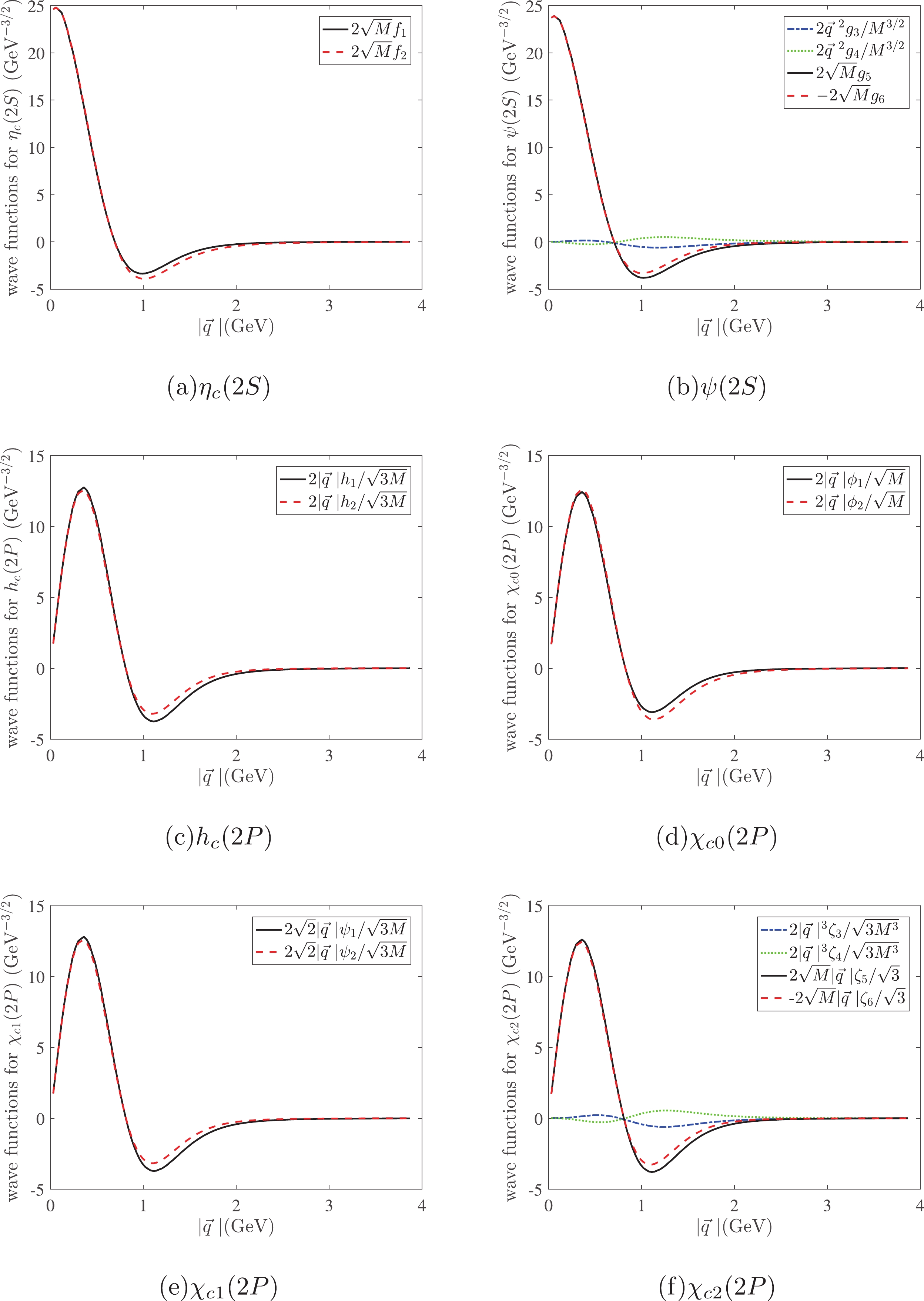

Figure 3.  (color online) Normalized radial wave functions of charmonium ($n = 2$).

The behaviors of the IWF $\xi_{00}$ and high-order corrections $\xi_{qx}$, i.e., the overlapping integrals of the wave functions of the initial and final bound states, are computed numerically and plotted in Figs. 4-5, where $\omega = v\cdot v_f = \frac{P\cdot P_f}{MM_f}$. These IWFs can be classified into four categories according to the configurations $nL$ of the initial and final states. They belong to the modes $1S\to 1S$, $1S\to 1P$, $1S\to 2S$, and $1S\to 2P$. In each mode, for example, in the processes $B_c\to\eta_c$ and $B_c\to J/\psi$, the behaviors of IWFs are virtually identical, except for their argument $\omega = v\cdot v_f$. This is because these decay processes are simply related by a rotation of the heavy-quark spin or the meson spin and this rotation is a symmetry transformation in the infinite-mass limit. Note that the infinite-mass limit is not used in this paper, but this spin-symmetry is reflected in the results automatically, as Figs. 4-5 show. This indicates that the spin-symmetry still holds, even though the initial and final states are both double-heavy mesons. Comparing the different modes, for example, where the final $\eta_c$ turns into $\eta_c(2S)$, the behaviors of IWFs differ significantly from before. Next, we will discuss these four modes one by one.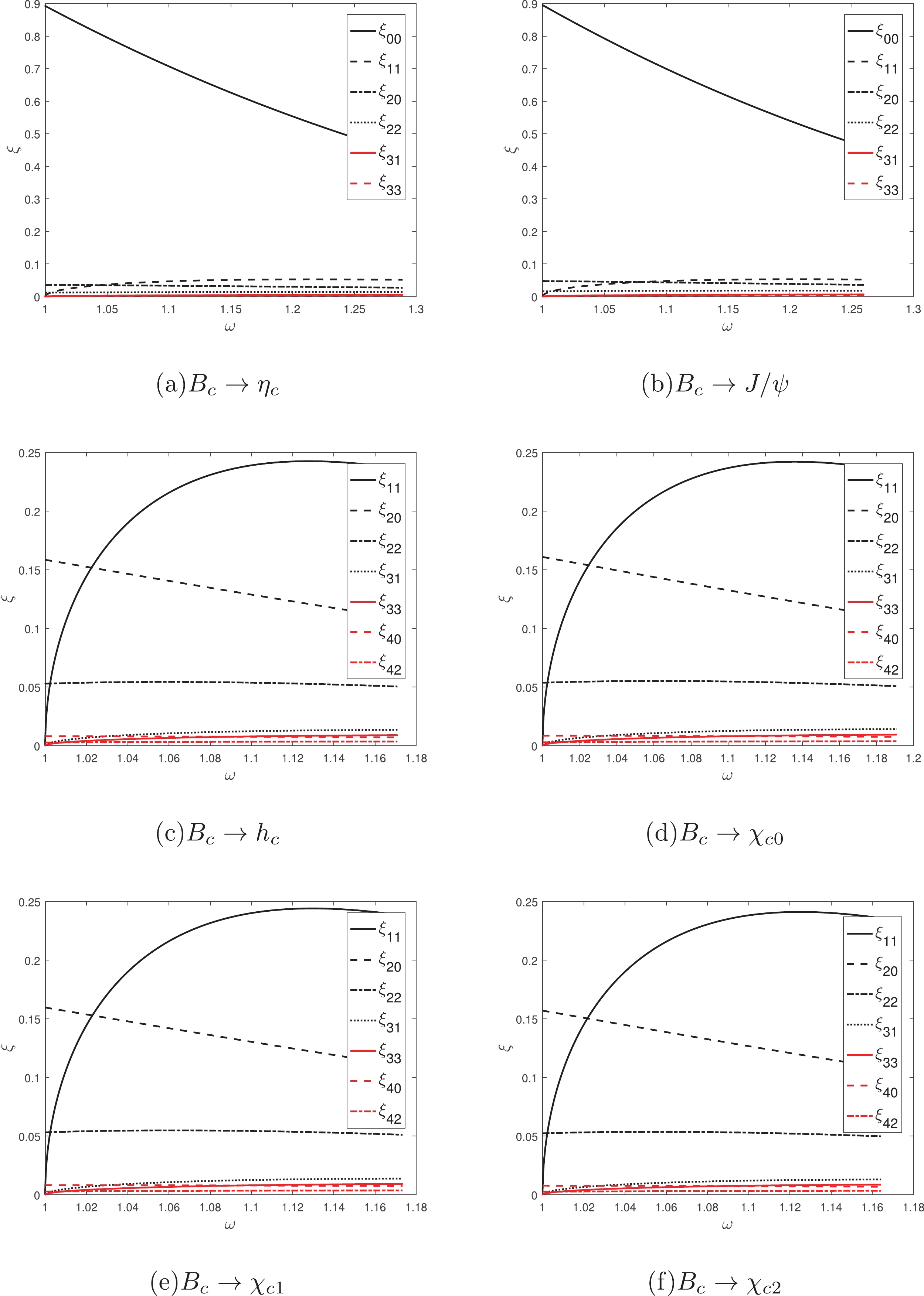

Figure 4.  (color online) IWF and high-order corrections $\xi_{qx}$ vs. $\omega$ for $B_c$ to charmonium ($n=1$), where $\omega=v\cdot v_f=\frac{P\cdot P_f}{MM_f}$. The solid line is the Isgur-Wise function, the dashed and dotted-dashed lines are the first order correction functions, the dotted line is the second order correction function, and so on, in every subfigure.

Figure 5.  (color online) IWF and high-order corrections $\xi_{qx}$ vs. $\omega$ for $B_c$ to charmonium ($n=2$), where $\omega=v\cdot v_f=\frac{P\cdot P_f}{MM_f}$. The meaning of each line type is the same as that in Fig. 4.

The mode $1S\to 1S$ has been extensively studied in HQET. $B_c$ and $\eta_c$ are related by the replacement $b\to c$, while $\eta_c$ and $J/\psi$ are related by the transformation $c^{\Uparrow}\to c^{\Downarrow}$ here. These two rotations (flavor and spin rotations) are symmetry transformations in the infinite-mass limit. Therefore, the radial wave functions of these mesons will be identical in this limit, and the corresponding IWF at zero recoil, i.e., $\xi(1)$ will be the same as the normalization formula of wave functions. It is very natural that $\xi(1) = 1$ in HQET. In this paper, we solve the full Salpeter equations without the infinite-mass limit, and the normalized radial wave function is approximated to $2\sqrt{M}f$ for the $1S$ state. The normalized wave functions have little difference for $\eta_c$ and $J/\psi$ (two dominant wave functions), which is consistent with Eq. (23). However, the discrepancy between $B_c$ and the former two is on the order of 30% (peak value), as Figs. 2(a)-2(c) show. This indicates that in the double-heavy system, the spin-symmetry holds, while the flavor-symmetry breaks. The quark and antiquark masses are on the same order of magnitude; therefore, the change in flavor will have a large effect. Although the analytical expressions (Eq. (20) and Eq. (22)) of the form factors parameterized by a single IWF $\xi_{00}$ are the same as those in HQET, these IWFs $\xi_{00}$ are not strictly unity at zero recoil in this paper, as Figs. 4(a)-4(b) show. The relativistic correction ($1/m_Q$ correction) reflected in IWF $\xi_{00}$ is approximately 10% at zero recoil, which is consistent with the estimate from HQET [2]. In the mode $1S\to 1S$, it is convenient to fit the IWF as

where $\rho^2$ is the slope parameter and c is the curvature parameter that characterizes the shape of the IWF. The slope by fitting is 2.25 in $B_c\to\eta_c$ and 2.38 in $B_c\to J/\psi$. These results agrees with the rule that the slope increases as the (reduced) mass becomes heavier [11, 31]. Note that the fitting Eq. (26) is only used to compare our slopes with other studies, but is not used elsewhere in this manuscript. The other functions $\xi_{qx}$ are the relativistic corrections to the form factors parameterized by a single IWF $\xi_{00}$. The more $\vec q\:'$ the correction function contains, the less contribution it makes. We may call the correction function with one relative momentum $\vec q\:'$ the first order correction, the correction function with two $\vec q\:'$ the second order correction, and so on. The values of $\xi_{11}$ are approximately 1/20 of those of $\xi_{00}$, as Figs. 4(a)-4(b) show. Because the decay width is proportional to the modular square of amplitude, the first order correction to the decay width may reach 1/10 of the leading order result, which is important for accurate calculation. Our previous study shows that the higher order relativistic corrections also have considerable contributions, and the total relativistic correction can reach approximately 20% at the level of decay width [43].

In the mode $1S\to 1P$, the configuration of the initial state is $1S$, while the configuration of the final state is $1P$. Their orbital angular momenta are different, so the symmetry transformations exist only between the final states, i.e., spin rotations. $\chi_{c0}$, $\chi_{c1}$, and $\chi_{c2}$ are spin triplet states that are related by the rotation of the total spin component (the component of total spin in the direction of orbital angular momentum), while $h_c$ and the former three are related by the transformation $c^{\Uparrow}\to c^{\Downarrow}$. These two spin rotations are symmetry transformations in the infinite-mass limit, so the normalized radial wave functions of these mesons will be identical. The infinite-mass limit is not adopted here, and the normalized radial wave functions of these mesons are approximated as $\frac{2|\vec q\:|h}{\sqrt{3M}},\frac{2|\vec q\:|\phi}{\sqrt{M}},\frac{2\sqrt{2}|\vec q\:|\psi}{\sqrt{3M}}$, and $\frac{2\sqrt{M}|\vec q\:|\zeta}{\sqrt 3}$ respectively, where $h, \phi, \psi$, and $\zeta$ are the independent components of the BS wave functions. Their numerical results are almost the same, as Figs. 2(d)-2(f) shows, which is consistent with Eq. (24). This indicates that the spin-symmetry holds in the P-wave charmonium, even though the quark and anti-quark have the same masses. Because the P-wave function contains a $\vec q\:$, $\xi_{00}$ disappears, and the IWF is $\xi_{11}$, whose behavior is obviously different from that of $\xi_{00}$. Because of the presence of $\cos\theta$, see Eq. (16), the IWF $\xi_{11}$ is zero at zero recoil, and it is enhanced kinematically, as Figs. 4(c)-4(e) shows. This behavior agrees with Ref. [37]. There is a kinematically suppressed factor $1/|\vec v_f|$ in the form factors Eq. (25); therefore, the behaviors of the leading order form factors are not purely dependent on $\xi_{11}$. Further, $\xi_{20}$ and $\xi_{22}$ are comparable with the leading order $\xi_{11}$, especially at zero recoil. $\xi_{22}$ is smaller than $\xi_{20}$ because of the factor $\cos^2\theta$. They decrease slowly when the momentum recoil increases; therefore, the relativistic corrections may be comparable with the nonrelativistic results in this mode. Although the other correction functions seem to be very small, they are still important for accurate calculation, just as in the mode $1S\to 1S$. For the final states $h_c$, $\chi_{c0}$, $\chi_{c1}$, and $\chi_{c2}$, the total relativistic corrections are 50%, 64%, 34%, and 14% at the level of decay width, respectively [43]. The total relativistic correction of $B_c\to\chi_{c2}$ is unusually small because the different order corrections cancel each other out. This can be seen in the following analysis of form factors.

In the mode $1S\to 2S$, the configuration of the initial state is different from that of the final state. Similarly, the only symmetry transformation is the spin rotation $c^{\Uparrow}\to c^{\Downarrow}$, which relates $\eta_c(2S)$ with $\psi(2S)$. Their normalized wave functions are almost the same, as Fig. 3(a)-3(b) shows, which is consistent with Eq. (23). The numerical results of the IWFs in this mode are negative. Although the signs of the IWFs do not affect the width, the negative values of the IWFs indicate that the negative parts of $2S$-wave functions play a primary role. The overlapping integral of wave functions $\int {\rm{d}}\vec q = \int\vec q\:^2\sin\theta {\rm{d}}|\vec q\:| {\rm{d}}\theta {\rm{d}}\phi$ contains a factor $\vec q\:^2$. It is suppressed when $|\vec q\:|<1$, while it is enhanced when $|\vec q\:|>1$. The negative parts of $2S$-wave functions are mostly in the range of $|\vec q\:|>1$, so the negative parts play a primary role in the overlapping integral. The IWF $\xi_{00}$ is increasing together with the momentum recoil, as Figs. 5(a)-5(b) show, and the leading order form factors have the same behaviors, according to Eqs. (20) and (22). The behaviors of other correction functions in this mode are similar to $1S\to 1S$, but they make more contributions here. For example, $\xi_{11}$ and $\xi_{20}$ are approximately one fifth and one eighth of $\xi_{00}$ at the maximum recoil, respectively. Therefore, the relativistic corrections become greater, and our previous study shows that they are approximately 19%–28% larger than those in the mode $1S\to 1S$ [43].

Compared with the mode $1S\to 1P$, the analysis of the symmetry and normalized wave functions is the same in $1S\to 2P$, as Figs. 5(c)-5(e) show. The IWF $\xi_{11}$ is also zero at zero recoil, but it increases more slowly. $\xi_{20}$ and $\xi_{22}$ are comparable with the IWF $\xi_{11}$, and they are no longer decreasing; in contrast, they increase as the momentum recoil increases. Therefore, the relativistic corrections may be more significant in this mode. They are approximately 10%–16% larger than those in the mode $1S\to 1P$ [43].

The above analysis of relativistic corrections is qualitative because the kinematic factors multiplied by the IWFs are different and complex. To discuss these relativistic corrections precisely, the form factors in these processes need to be calculated by different order corrections in turn. These numerical results are compared with those calculated using the instantaneous Bethe-Salpeter method directly, as Figs. 6-13 show. In these Figs, $t\equiv(P-P_f)^2$ is the momentum transfer and $t_m$ is the maximum of t, so $t_m-t = 2MM_f(v\cdot v'-1)$. The circle-solid line (BSE) denotes the form factor calculated using the instantaneous Bethe-Salpeter method directly, and we regard it as the more precise result because this method is almost covariant; the solid line denotes the leading order (LO) of the form factor calculated only using the IWF; the dashed line denotes the result with the IWF and first order (1st) correction; the dotted-dashed line denotes the result with the IWF and the first and second order (2nd) corrections; the dotted line denotes the result with IWF and the first, second, and third order (3rd) corrections.

Figure 6.  (color online) The form factors of $B_c\to\eta_c,J/\psi$ calculated using the IWFs and instantaneous BS method, where $t\equiv(P-P_f)^2$ is the momentum transfer and $t_m-t=2MM_f(v\cdot v'-1)$. The circle-solid line denotes the form factor calculated using the instantaneous Bethe-Salpeter method directly; the solid line denotes the leading order of the form factor calculated only using the IWF; the dashed line denotes the result with the IWF and first order correction; the dotted-dashed line denotes the result with the IWF and the first and second order corrections; the dotted line denotes the result with the IWF and the first, second, and third order corrections.

Figure 7.  (color online) The form factors of $B_c\to h_c,\chi_{c0}$ calculated using the IWFs and instantaneous Bethe-Salpeter method, where $t\equiv(P-P_f)^2$ is the momentum transfer and $t_m-t=2MM_f(v\cdot v'-1)$. The meaning of each line type is the same as that in Fig. 6.

Figure 8.  (color online) The form factors of $B_c\to \chi_{c1}$ calculated using the IWFs and instantaneous Bethe-Salpeter method, where $t\equiv(P-P_f)^2$ is the momentum transfer and $t_m-t=2MM_f(v\cdot v'-1)$. The meaning of each line type is the same as that in Fig. 6.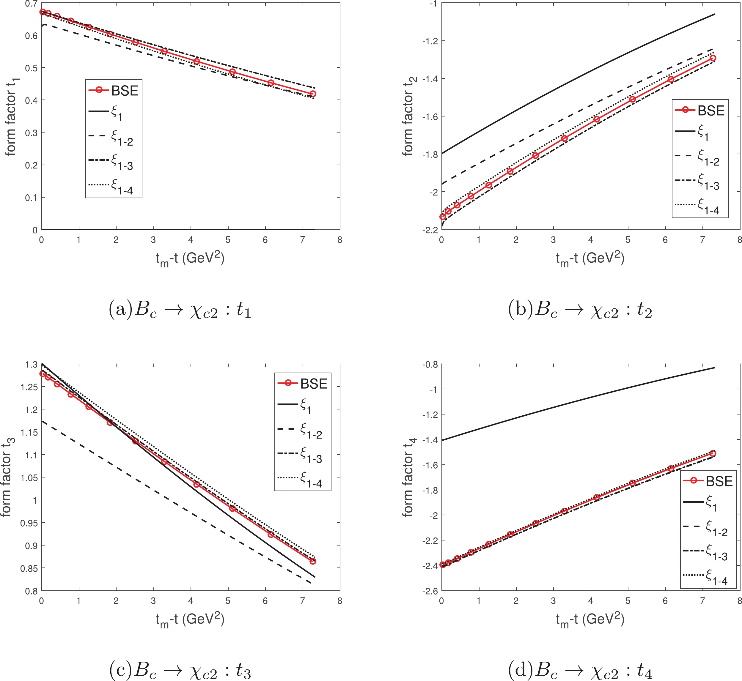

Figure 9.  (color online) The form factors of $B_c\to \chi_{c2}$ calculated using the IWFs and instantaneous Bethe-Salpeter method, where $t\equiv(P-P_f)^2$ is the momentum transfer and $t_m-t=2MM_f(v\cdot v'-1)$. The meaning of each line type is the same as that in Fig. 6.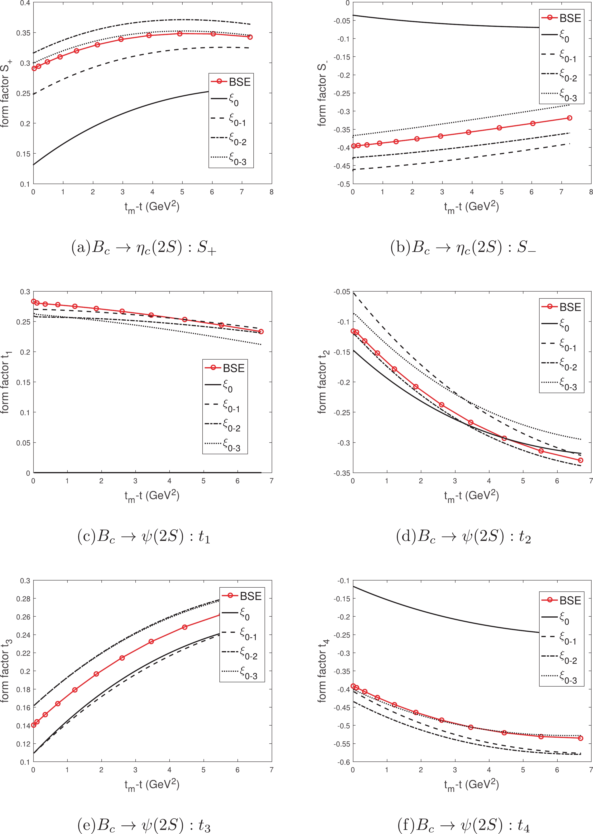

Figure 10.  (color online) The form factors of $B_c\to\eta_c(2S),\psi(2S)$ calculated using the IWFs and instantaneous Bethe-Salpeter method, where $t\equiv(P-P_f)^2$ is the momentum transfer and $t_m-t=2MM_f(v\cdot v'-1)$. The meaning of each line type is the same as that in Fig. 6.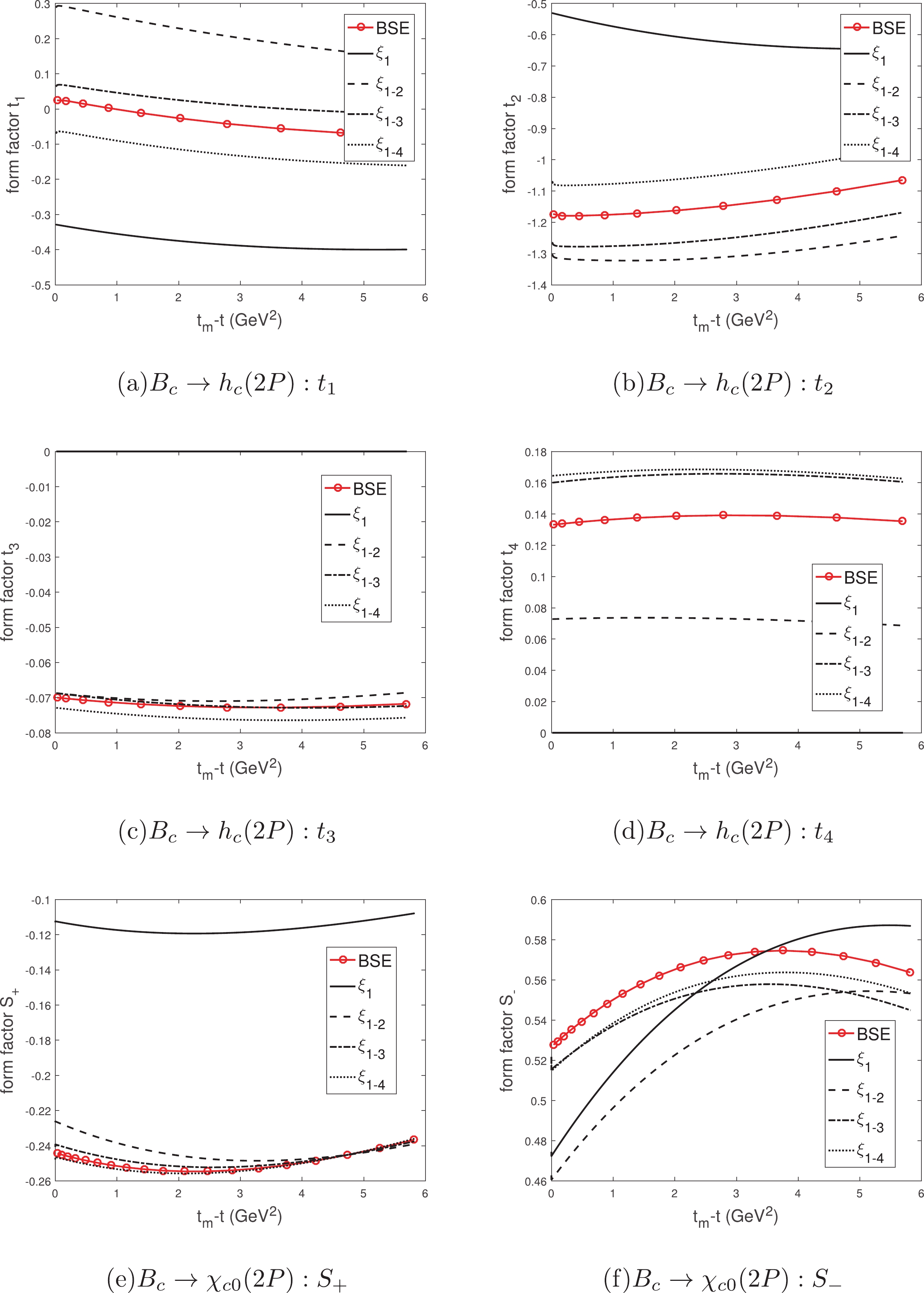

Figure 11.  (color online) The form factors of $B_c\to h_c(2P),\chi_{c0}(2P)$ calculated using the IWFs and instantaneous Bethe-Salpeter method, where $t\equiv(P-P_f)^2$ is the momentum transfer and $t_m-t=2MM_f(v\cdot v'-1)$. The meaning of each line type is the same as that in Fig. 6.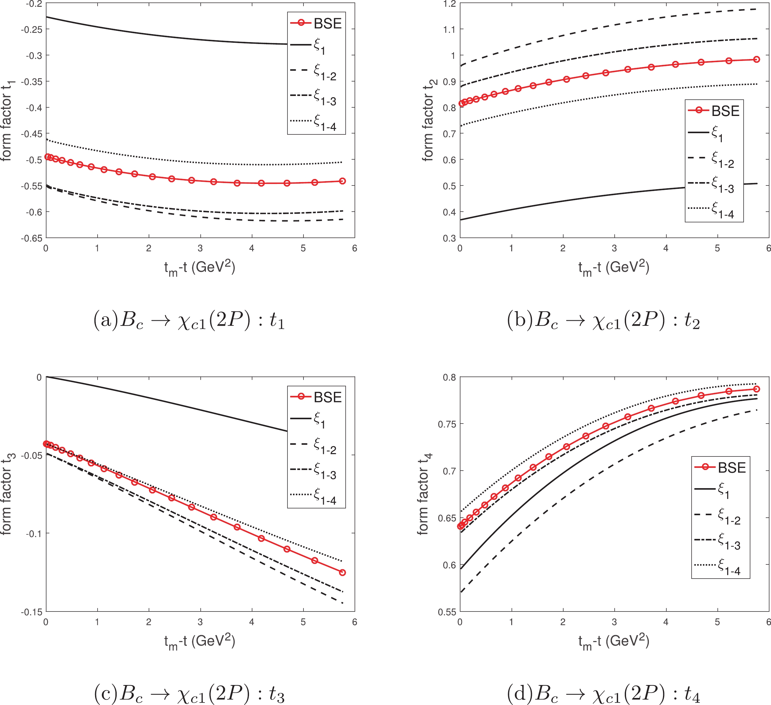

Figure 12.  (color online) The form factors of $B_c\to \chi_{c1}(2P)$ calculated using the IWFs and instantaneous Bethe-Salpeter method, where $t\equiv(P-P_f)^2$ is the momentum transfer and $t_m-t=2MM_f(v\cdot v'-1)$. The meaning of each line type is the same as that in Fig. 6.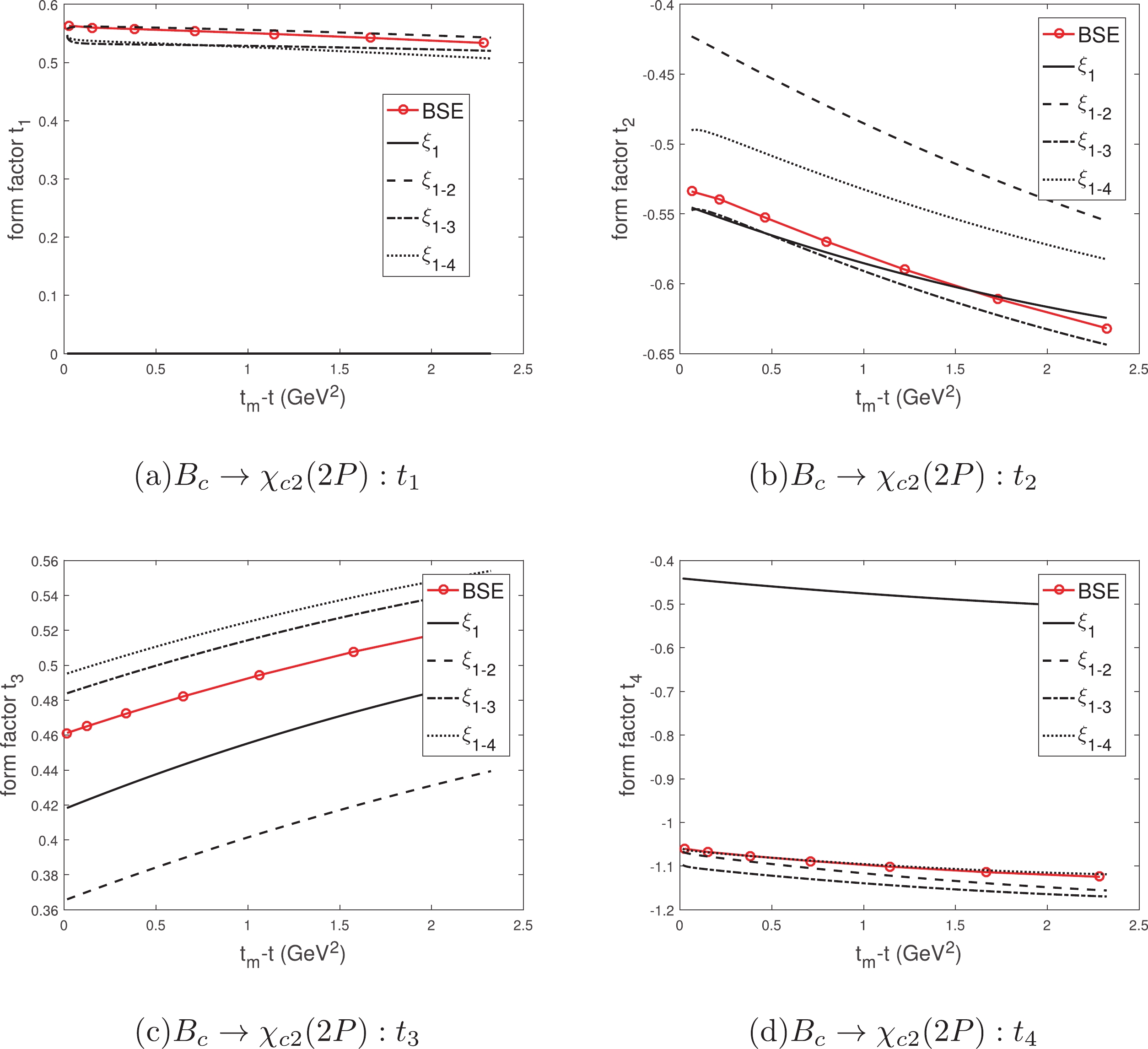

Figure 13.  (color online) The form factors of $B_c\to \chi_{c2}(2P)$ calculated usingt he IWFs and instantaneous Bethe-Salpeter method, where $t\equiv(P-P_f)^2$ is the momentum transfer and $t_m-t=2MM_f(v\cdot v'-1)$. The meaning of each line type is the same as that in Fig. 6.

For the process $B_c\to\eta_c$, as Figs. 6(a)-6(b) show, there is a gap between the leading order $S_+$ and the result from the BSE. The $S_+$ with the 1st correction is close to the BSE. When the 3rd correction is taken into account, the result becomes very accurate. The difference between the LO $S_-$ and the BSE is slightly larger, but because of the small contribution of $S_-$ to the decay width, the leading order results may be approximate. Although the high order corrections do not make $S_-$ and BSE exactly the same, they become closer. For the process $B_c\to J/\psi$, as Figs. 6(c)-6(f) show, the form factor $t_3$ makes the main contribution to the decay width. The LO $t_3$ has a slight gap with the BSE, and the result with high order corrections is more accurate. The LO $t_1$ is zero, which agrees with HQET, see Eq. (22), but is far from the BSE. The LO $t_2$ and $t_4$ are also different from the BSE. The high order corrections bring them closer to the BSE, of which the 1st correction is the most important one. In the mode $1S\to 1S$, the leading order form factors, which are parameterized by a single IWF $\xi_{00}$, may be approximate, but the high order corrections can make the result more precise. Note that the accurate result of $t_1$ cannot be obtained by correcting $\xi_{00}$; therefore, we need to introduce new high-order correction functions.

For the process $B_c\to h_c$, as Figs. 7(a)-7(d) show, the form factor $t_2$ makes the main contribution to the decay width. The LO $t_2$ is slightly different from the BSE. The 1st, 2nd, and 3rd corrections are not small, but they almost cancel each other out. These corrections bring $t_2$ closer to the BSE. The LO $t_3$ and $t_4$ are zero, which can be used to examine our method. The $t_1$, $t_2$, and $t_4$ with the 1st correction are still quite different from the BSE; therefore, higher order corrections are necessary. For the process $B_c\to \chi_{c0}$, as Figs. 7(e)-7(f) show, the difference between the LO $S_+$ and the BSE is large. At the least, the 1st correction needs to be considered to reach an approximate result, although the $S_-$ with the 1st correction is not accurate enough. The higher order corrections can make the results more accurate. For the process $B_c\to \chi_{c1}$, as Figs. 8(a)-8(d) show, the form factor $t_2$ makes the main contribution to the decay width. The 1st corrections are great, except $t_4$. The higher order corrections are small but still important for accurate calculation. For the process $B_c\to \chi_{c2}$, as Figs. 9(a)-9(d) show, the form factor $t_3$ makes the main contribution to the decay width. The LO $t_3$ is close to the BSE, and the high order corrections almost cancel each other out. This leads to the unusually small result of the total relativistic correction. The 1st correction brings $t_1$, $t_2$, and $t_4$ closer to the BSE, but it makes the main form factor $t_3$ farther from the BSE. The result may be more imprecise if only the IWF and 1st correction are considered, so the higher-order corrections are very important. At zero recoil, the IWF $\xi_{11}$ is zero and the kinematic factor $(v\cdot v_f)/|\vec v_f|$ will lead to the divergence; see Eq. (25). However, most LO form factors are limited values at zero recoil. In general, the relativistic corrections are large, and the 1st corrections can only derive the approximate results in the mode $1S\to 1P$.

In the modes $1S\to 2S$ and $1S\to 2P$, the form factors are no longer depressed, but are instead slightly enhanced. The relativistic corrections are similar to those discussed above, but are greater and more complicated, as Figs. 10-13 show. In general, there are large gaps between the leading order form factors and those from the BSE directly. The newly introduced high-order correction functions make significant contributions to these relativistic corrections.

In this work, we examine the validity of the heavy quark effective theory for double heavy mesons using the instantaneous Bethe-Salpeter method from a phenomenological perspective. With some approximations, all form factors are parameterized by some universal functions $\xi_{qx}$. These functions are calculated using the overlapping integrals of the phenomenological BS wave functions for the initial state and the final state. We reproduce the classical formulas of the HQET, in which the leading order form factors are parameterized by a single Isgur-Wise function $\xi_{00}$. The heavy quark limit is not adopted here; therefore, the IWF $\xi_{00}$ in this paper is the corrected IWF in HQET, which contains the relativistic correction ($1/m_Q$ correction). The IWF $\xi_{00}$ is not strictly equal to unity numerically at zero recoil, i.e., $\xi_{00}(1)\neq 1$.

We choose the semileptonic $B_c$ decays to charmonium to calculate the numerical results of the Isgur-Wise functions and form factors, where the final states include $1S$, $1P$, $2S$, and $2P$. The form factors parameterized by a single corrected IWF $\xi_{00}$ deviate seriously from the full ones, especially when involving the excited states. The deviation requires the introduction of more non-perturbative universal functions $\xi_{qx} (q\neq 0)$. These functions $\xi_{qx} (q\neq 0)$ are the relativistic corrections ($1/m_Q$ corrections) to the leading order results. These functions $\xi_{qx}$ primarily depend on the configurations $nL$ of the initial and final states; thus, they are universal for each mode. These results can simplify the calculations of form factors. This simplification can be generalized to other modes, including but not limited to $1S\to 1P$, $1S\to 2S$, and $1S\to 2P$, which are studied in this paper. We conclude that the HQET is applicable to these decays in this paper from a phenomenological aspect, but the higher order correction functions $\xi_{qx}(q\neq 0)$ provide large relativistic corrections ($1/m_Q$ corrections) and must be introduced.

The BS equation for a quark-antiquark bound state generally is written as [46]

where $p_1,p_2;m_1,m_2$ are the momenta and masses of the quark and antiquark, respectively; $\chi_P(q)$ is the BS wave function with total momentum P and relative momentum q; and $V(P,k,q)$ is the kernel between the quark-antiquark in the bound state. P and q are defined as

We divide the relative momentum q into two parts, $q_{P_{||}}$ and $q_{P_{\perp}}$, a part parallel to and one orthogonal to P, respectively,

where $q_{P_{||}}^{\mu}\equiv(P\cdot q/M^2)P^{\mu},\; q_{P_{\perp}}^{\mu}\equiv q^{\mu}-q_{P_{||}}^{\mu}$, and M is the mass of the relevant meson. Correspondingly, we have two Lorentz-invariant variables

If we introduce two notations as follows

then the BS equation can take the following form:

The propagators of the relevant particles with masses $m_1$ and $m_2$ can be decomposed as

with

where $i = 1,2$ for a quark and antiquark, respectively, and $J(i) = (-1)^{i+1}$.

Then, the instantaneous Bethe-Salpeter equation can be decomposed into the coupled equations

The instantaneous kernel has the following form,

especially when the two constituents of the meson are very heavy. The kernel we use contains a linear scalar interaction for color-confinement, a vector interaction for one-gluon exchange, and a constant $V_0$ as a "zero-point," i.e.,

where $\lambda$ is the "string constant" and $\alpha_s(r)$ is the running coupling constant. To avoid the infrared divergence, a factor ${\rm e}^{-\alpha r}$ is introduced, i.e.,

In momentum space, the kernel reads:

where

The fitted parameters are $a = e = 2.7183$, $\alpha = 0.06$ GeV, $\lambda = 0.21$ ${\rm GeV}^2$, and $\Lambda_{\rm QCD} = 0.27$ GeV; $V_0$ is fixed by fitting the mass of the ground state. With these parameters, the mass spectra, decay constants, and some branching fractions of the double heavy mesons, including $B_c$, charmonium, and bottomium, can be obtained. These results are in good agreement with the experimental data. More details can be found in the literature [47, 48].

The instantaneous Bethe-Salpeter wave function for $2^{++}$ state mesons has the general form [41]

with

The wave function corresponding to the positive projection has the form

where

If the masses of the quark and antiquark are equal, the normalization condition is