What can a heavy ${{U(1)}_{\bf B-L} \; {Z^\prime}}$ boson do to the muon ${{(g-2)}_{\mu}}$ anomaly and to a new Higgs boson mass?

It is unquestionable that the Standard Model (SM) is a successful framework that accurately describes the phenomenology of particle physics up to the highest energy scales probed by collider measurements so far. In fact, contemporary direct searches for new physics or indirect probes (e.g., via flavor anomalies) have been showing an increasingly puzzling consistency with the SM predictions. However, it is equally true that the SM has its weaknesses, and several open questions are yet to be understood. One such weakness is a missing explanation of tiny neutrino masses confirmed by flavor-oscillation experiments. The minimal way of addressing this problem is by adding heavy Majorana neutrinos, for realizing a seesaw mechanism [1-3]. However, the mere introduction of an arbitrary number of heavy neutrino generations can raise new questions, in particular, how such a new scale is generated from a more fundamental theory.

Among the simplest ultraviolet (UV) complete theories that dynamically address this question is the minimal gauge-${U}(1)_{\rm{B - L}}$ extension of the SM [4-7], traditionally dubbed as the B-L-SM. As its name suggests, the B-L-SM promotes an accidental conservation of the difference between the baryon (B) and lepton (L) numbers in the SM to a fundamental local Abelian symmetry group. Furthermore, such a ${U}(1)_{\rm{B - L}}$ symmetry can be embedded into larger groups, e.g., ${SO}({10})$ [8-12] or ${E}_{{6}}$ [13-15], making the B-L-SM well motivated by Grand Unified Theories (GUTs). The presence of three generations of right-handed neutrinos also ensures a framework free of anomalies, with their mass scale developed once the ${U}(1)_{\rm{B - L}}$ is broken by the VEV of a complex SM-singlet scalar field, simultaneously giving mass to the corresponding $Z^\prime$ boson.

The cosmological implications of the B-L-SM are also relevant. First, the presence of an extended neutrino sector implies the existence of a sterile state that can be ${\rm{keV}}$- to ${\rm{TeV}}$-scale Dark Matter candidate [16]. Particularly, it can be stabilized by imposing a ${\mathbb Z}_2$ parity as it was done, e.g., in Refs. [17-19]. The ${U}(1)_{\rm{B - L}}$ model with sterile neutrino Dark Matter can also explain the observed baryon asymmetry via the leptogenesis mechanism (see Refs. [20-24] for details). As was mentioned earlier, the B-L-SM features an extended scalar sector with a complex SM-singlet state $\chi$, which, besides enriching the Higgs sector with a new potentially visible state, can cure the well-known metastability of the electroweak (EW) vacuum in the SM [25-27]. Indeed, it was shown in Ref. [28] that an additional physical scalar with a mass beyond a few hundred ${\rm{GeV}}$ can stabilize the Higgs vacuum all the way up to the Planck scale. In the framework of the B-L-SM, a complete study of the scalar sector was performed in Ref. [29], where the vacuum stability conditions valid at any Renormalization Group (RG) scale were derived. Last but not least, the presence of the complex SM-singlet $\chi$ interacting with a Higgs doublet typically enhances the strength of the EW phase transition, potentially converting it into a strong first-order one [30].

Another open question that has no solution in the SM framework is the discrepancy between the measured anomalous magnetic moment of the muon, $a_\mu^{{\exp}} \equiv \displaystyle\frac{1}{2} (g-2)^{{\exp}}_\mu$, and its theoretical prediction, $a_\mu^{\rm{SM}} \equiv \displaystyle\frac{1}{2} (g-2)^{\rm{SM}}_\mu$, which reads [31, 32]

with the numbers in the brackets denoting experimental and theoretical errors, respectively. This represents a tension of $3.3$ standard deviations from the combined $1 \sigma$ error and calls for new physics effects beyond the SM theory. In a recent work [33], it was further claimed that the SM higher order perturbative corrections cannot explain $\Delta a_\mu$. A popular explanation for such an anomaly resides in low-scale supersymmetric models [34-44] where smuon-neutralino and sneutrino-chargino loops can explain the discrepancy (1). However, this solution is by no means unique, and radiative corrections with new gauge bosons can also contribute to the theoretical value of the muon anomaly [45-48]. This is indeed the case for the B-L-SM, or its SUSY version [49-51], where a new $Z^\prime$ gauge boson can explain $\Delta a_\mu$.

In a recent work [52], the impact of LHC searches for a light $Z^\prime$ boson, i.e., with mass ranging from $0.2\; {\rm{GeV}}$ to $200\; {\rm{GeV}}$, was thoroughly investigated. The current collider bounds are available from the ATLAS [53] and CMS [54] searches for Drell-Yan $Z^\prime$ production decaying into di-leptons, i.e., $pp \to Z^\prime \to ee,\mu \mu$. In the current work, we perform a complementary study where, for heavy (TeV-scale) $Z^\prime$ masses, the combined effect of the electroweak precision and Higgs observables and collider constraints on the $pp \to Z^\prime \to ee,\mu \mu$ channel is investigated. We analyze whether the existing LHC constraints leave any room for partially explaining the $(g-2)_\mu$ anomaly and the impact it has on the model parameters and other physical observables, such as the ${U}(1)_{\rm{B - L}}$ gauge coupling $g_{\rm{B - L}}$, the kinetic mixing parameter $g_{{\rm{YB}}}$ , and the extra scalar and $Z^\prime$ boson masses. Furthermore, with the current muon $(g-2)_\mu$ experiment E989 at Fermilab [55], it will be possible to either confirm or eliminate, at least partially, the currently observed discrepancy, making our work rather timely.

The article is organized as follows. In Section II, we provide a brief description of the B-L-SM structure focusing on the basic details of scalar and gauge boson mass spectra and mixing. In Section III, a detailed discussion of the numerical analysis is provided. In particular, we outline the methods and tools used in our numerical scans as well as the most relevant phenomenological constraints leading to a selection of a few representative benchmark points. In addition, the numerical results for correlations of the $Z^\prime$ production cross section times the branching ratio for light leptons versus the model parameters and the muon $(g-2)_\mu$ are presented. Finally, Section IV provides a short summary of our main results.

In this section, we highlight the essential features of the minimal ${U}(1)_{\rm{B - L}}$ extension of the SM that are relevant to our analysis. Essentially, the minimal B-L-SM is a Beyond the Standard Model (BSM) framework, containing three new ingredients: 1) a new gauge interaction, 2) three generations of right handed neutrinos, and 3) a complex scalar SM-singlet. The first one is well motivated in various GUT scenarios [8-15]. However, if a family-universal symmetry such as ${U}(1)_{\rm{B - L}}$ is introduced without changing the SM fermion content, chiral anomalies involving the ${U}(1)_{\rm{B - L}}$ external legs would be generated. A new sector of additional three ${\rm B-L}$ charged Majorana neutrinos is essential for anomaly cancellation. In addition, the SM-like Higgs doublet, H, carries neither the baryon nor the lepton number and therefore does not participate in the breaking of ${U}(1)_{\rm{B - L}}$. It is then necessary to introduce a new scalar singlet, $\chi$, solely charged under ${U}(1)_{\rm{B - L}}$, whose VEV breaks the ${\rm B-L}$ symmetry on the scale $\left \langle {\chi} \right \rangle > \left \langle {H} \right \rangle$. It is also this breaking scale that generates masses for heavy neutrinos. The particle content and charges of the minimal ${U}(1)_{\rm{B - L}}$ extension of the SM are summarized in Table 1.

	${SU }({3})_{\rm{C} }$	${SU }({2})_{\rm{L} }$	${U}(1)_{\rm{Y} }$	${U}(1)_{\rm{B - L} }$
$q_{\rm{L}}$	${\bf{3}}$	${\bf{2}}$	$1/6$	$1/3$
$u_{\rm{R}}$	${\bf{3}}$	${\bf{1}}$	$2/3$	$1/3$
$d_{\rm{R}}$	${\bf{3}}$	${\bf{1}}$	$-1/3$	$1/3$
$\ell_{\rm{L}}$	${\bf{1}}$	${\bf{2}}$	$-1/2$	$-1$
$e_{\rm{R}}$	${\bf{1}}$	${\bf{1}}$	$-1$	$-1$
$\nu_{\rm{R}}$	${\bf{1}}$	${\bf{1}}$	$0$	$-1$
H	${\bf{1}}$	${\bf{2}}$	$1/2$	$0$
$\chi$	${\bf{1}}$	${\bf{1}}$	$0$	$2$

Table 1.  Fields and their quantum numbers in the minimal B-L-SM. The last two columns represent the weak and ${\rm B-L}$ hypercharges, which we denote as Y and $Y_{\rm{B - L}}$ throughout the text.

The scalar potential of the B-L-SM reads

where H and $\chi$ are the Higgs doublet and the complex SM-singlet, respectively, whose real-valued components can be cast as

While v and x are the vacuum expectation values (VEVs) describing the classical ground state configurations of the theory, h and $h^\prime$ represent radial quantum fluctuations around the minimum of the potential. There are four Goldstone directions denoted as $\omega_1$, $\omega_2$, z , and $z^\prime$ , which are absorbed into the longitudinal modes of the W, Z, and $Z^\prime$ gauge bosons once spontaneous symmetry breaking (SSB) takes place. The scalar potential (2) is bounded from below (BFB) whenever the conditions [29]

are satisfied and the electric charge conserving vacuum

is stable. Resolving the tadpole equations with respect to the VEVs, one obtains

which imply, together with the BFB conditions (4), that

While the signs of $\lambda_1$ and $\lambda_2$ are positive, the inequalities (7) put further constraints on the signs of $m^2$, $\mu^2$, and $\lambda_3$ according to Table 2. We see that if $\lambda_3$ is positive, a minimum in the scalar potential can emerge, provided that both $\mu^2$ and $m^2$ are not simultaneously positive. However, in our studies, we have considered the $\lambda_3 > 0$ solution in the last column of Table 2, where both the ${SU}({2})_{\rm{L}}$ isodoublet and the complex singlet mass parameters are negative.

	$\mu^2> 0$ $m^2> 0$	$\mu^2> 0$ $m^2< 0$	$\mu^2< 0$ $m^2> 0$	$\mu^2< 0$ $m^2< 0$
$\lambda_3< 0$	×	$\checkmark$	$\checkmark$	$\checkmark$
$\lambda_3> 0$	×	×	×	$\checkmark$

Table 2.  Signs of parameters in the potential (2). While the $\checkmark$ symbol indicates the solutions of the tadpole conditions (7), which, together with the positively-definite scalar mass spectrum, correspond to a minimum of the scalar potential, the symbol × indicates unstable configurations.

Taking the Hessian matrix and evaluating it in the vacuum (5), one obtains

which can be rotated to the mass eigenbasis as

where the eigenvalues are

and the orthogonal rotation matrix ${{O}}$ reads

The physical basis vectors $h_1$ and $h_2$ can then be written in terms of the gauge eigenbasis ones h and $h^\prime$ , as follows:

In this article, we consider scenarios where ${U}(1)_{\rm{B - L}}$ is broken above the EW-scale, such that $x > v$. In the case of decoupling $v/x\ll 1$, the scalar masses and the mixing angle become particularly simple,

which represents a good approximation for most of the phenomenologically consistent points in our numerical analysis discussed below.

The gauge boson and Higgs kinetic terms in the B-L-SM Lagrangian read

where $F^{\mu \nu}$ and $F^{\prime \mu \nu}$ are the standard ${U}(1)_{\rm{Y}}$ and ${U}(1)_{\rm{B - L}}$ field strength tensors, respectively,

written in terms of the gauge fields $A_\mu$ and $A_\mu^\prime$, respectively. The $\kappa$ parameter in Eq. (14) represents the ${U}(1)_{\rm{Y}} \times {U}(1)_{\rm{B - L}}$ gauge kinetic mixing, while the Abelian part of the covariant derivative reads

with $g_1$ and $g_1^\prime$ being the ${U}(1)_{\rm Y}$ and ${\rm{U}}(1)_{\rm{B - L}}$ gauge couplings, respectively; the Y and ${\rm B-L}$ charges are specified in Table 1.

In order to study the kinetic mixing effects on physical observables, it is convenient to rewrite the gauge kinetic terms in the canonical form, i.e.,

A generic orthogonal transformation in the field space does not eliminate the kinetic mixing term. Thus, to satisfy Eq. (17), an extra non-orthogonal transformation should be imposed, such that Eq. (17) is realized. Taking $\kappa = \sin \alpha$, a suitable redefinition of fields $\{A_\mu,A_\mu^\prime\}$ into $\{B_\mu, B_\mu^\prime\}$ that eliminates $\kappa$-term according to Eq. (14) can be cast as

such that in the limit of no kinetic-mixing, $\alpha = 0$. Note that this transformation is generic and valid for any basis in the field space. The transformation (18) results in a modification of the covariant derivative that acquires two additional terms encoding the details of the kinetic mixing, i.e.,

where the gauge couplings take the form

which is the standard convention in literature. The resulting mixing between the neutral gauge fields including $Z^\prime$ can be represented as follows

where $\theta_W$ is the weak mixing angle, and $\theta^\prime_W$ is defined as

in terms of g and $g_{\rm{Y}}$, which are the ${SU}({2})_{\rm{L}}$ and ${U}(1)_{\rm{Y}}$ gauge couplings, respectively. In the physically relevant limit, $v/x \ll 1$, the above expression greatly simplifies, leading to

up to $(v/x)^3$ corrections. In the limit of no kinetic mixing, i.e., $g_{{\rm{YB}}} \to 0$, there is no mixture of $Z^\prime$ and SM gauge bosons.

Note that the kinetic mixing parameter $\theta_W^\prime$ has rather stringent constraints from Z pole experiments, both at the Large Electron-Positron Collider (LEP) [56] and the Stanford Linear Collider (SLC) [57], restricting its value to be smaller than $10^{-3}$ approximately, which we set as an upper bound in our numerical analysis. Expanding the kinetic terms $\left| {D_\mu H} \right|^2 + \left| {D_\mu \chi} \right|^2$ around the vacuum, one can extract the following mass matrix for vector bosons

whose eigenvalues read

corresponding to a physical photon and $W^\pm$ bosons as well as

for two neutral massive vector bosons, with one of them, not necessarily the lightest, representing the SM-like Z boson. It follows from LEP and SLC constraints on $\theta_W^\prime$ that Eq. (23) also implies that either $g_{{\rm{YB}}}$ or the ratio ${v}/{x}$ are small. In this limit, Eq. (26) simplifies to

where $m_{Z^\prime}$ depends only on the SM-singlet VEV x and on the ${U}(1)_{\rm{B - L}}$ gauge coupling and will be attributed to a heavy $Z^\prime$ state, while the light Z-boson mass corresponds to its SM value.

One of the key features of the B-L-SM is the presence of non-zero neutrino masses. In its minimal version, such masses are generated via a type-I seesaw mechanism. The Yukawa Lagrangian of the model reads

Notice that Majorana neutrino mass terms of the form $M \overline{\nu_{\rm{R}}^c} \nu_{\rm{R}}$ would explicitly violate the ${U}(1)_{\rm{B - L}}$ symmetry and are therefore not present. In Eq. (28), $Y_u$, $Y_d$ and $Y_e$ are the $3 \times 3$ Yukawa matrices that reproduce the quark and charged lepton sector of the SM, while $Y_\nu$ and $Y_\chi$ are the new Yukawa matrices responsible for the generation of neutrino masses and mixing. In particular, one can write

for light $\nu_l$ neutrino masses, whereas the heavy $\nu_h$ ones are given by

where we have assumed a flavor diagonal basis. Note that the smallness of light neutrino masses implies that either the x VEV is very large or (if we fix it to be at the ${\cal O}({\rm{TeV}})$ scale and ${{Y}}_\chi \sim {\cal O}(1)$) the corresponding Yukawa coupling should be small, ${{Y}}_\nu < 10^{-6}$. It is clear that the low scale character of the type-I seesaw mechanism in the minimal B-L-SM is faked by small Yukawa couplings to the Higgs boson. A more elegant description was proposed in Ref. [58] where small SM neutrino masses naturally result from an inverse seesaw mechanism. In this work, however, we will not study the neutrino sector, and thus, for an improved efficiency of our numerical analysis of $Z^\prime$ observables, it will be sufficient to fix the Yukawa couplings to ${{Y}}_\chi = 10^{-1}$ and ${{Y}}_\nu = 10^{-7}$ values such that the three lightest neutrinos lie in the sub-eV domain.

To assess the phenomenological viability of the minimal B-L-SM, we have developed a scanning routine that sequentially calls publicly available software tools in order to numerically evaluate physical observables and confront them against experimental data. Analytical expressions for such observables are calculated in SARAH 4.13.0 [59, 60] and then imported to SPheno 4.0.3 [61, 62], which is a spectrum generator where masses and mixing angles, EW precision observables, the muon anomalous magnetic moment as well as a number of decay widths and branching fractions are numerically evaluated. In addition, various theoretical constraints, such as the positivity of the one-loop mass spectrum and unitarity, are taken into account. As a first step, our scanning routine randomly samples parameter space points according to the ranges in Table 3. As can be seen from Eq. (13), $\lambda_1$ varies in a rather narrow domain in comparison to $\lambda_{2,3}$ , to comply with the experimental data on the SM Higgs mass (in the limit of large singlet VEV). In particular, provided that SPheno computes the SM Higgs boson mass in a two-loop order, the tree-level quantity $v \sqrt{2 \lambda_1}$ must not be too far from ${\cal O}(125\; {\rm{GeV}})$ for most of the valid points. In fact, we have verified that valid points typically require $\lambda_1 \sim {\cal O}(0.12 - 0.14)$, with a few cases where quantum corrections are somewhat larger. For the singlet VEV x, we scan over all its potentially phenomenologically interesting ranges, covering both large and small $Z’$ masses and both heavy and light second Higgs bosons. In particular, we aim at exploring a specific domain in the parameter space where a heavy $Z’$ is still compatible with a relatively light $h_2$. As we will discuss below, our results demonstrate that a $Z’$ boson with mass up to 10 TeV is still compatible with sub-TeV second Higgs state in the considered BL-SM.

$\lambda_{1}$	$\lambda_{2,3}$	$g_{\rm{B-L}}$	$g_{\rm{YB}}$	$x/{\rm{TeV}}$
$[10^{-2},\, 10^{0.5} ]$	$[ 10^{-8},\, 10 ]$	$[ 10^{-8},\, \sqrt{4\pi}]$	$[ 10^{-8},\, \sqrt{4\pi} ]$	$[ 0.5,\, 20.5 ]$

Table 3.  Parameter scan ranges used in our analysis. Note that the value of $\lambda_1$ is mostly constrained by the tree-level Higgs boson mass given in Eq. (13).

In the B-L-SM, new physics (NP) contributions to $a_\mu$, denoted as $\Delta a_\mu^{\rm{NP}}$ in what follows, can emerge from the diagrams containing $Z^\prime$ or $h_2$ propagators. In this article, we study whether the muon anomalous magnetic moment can be at least partially explained by the model under consideration. Each parameter space point generated with our routine undergoes a sequence of tests before getting accepted. The very first layer of phenomenological checks is done by SPheno, which promptly rejects any scenario with tachyonic scalar masses. If the positivity of the squared scalar spectrum is assured, SPheno verifies whether unitary constraints are also fulfilled. For details, see the pioneering work in [63] or the discussion in [64]. The presence of new bosons in the theory can induce large deviations in the EW precision observables. Typically, the most stringent constraints emerge from the oblique $S,T,U$ parameters [65-67], which are calculated by SPheno. In Fig. 1, we present the results for the EW oblique corrections in the $ST$ (upper row) and $TU$ (lower row) planes, together with their correlations with respect to the ${U}(1)_{\rm{B - L}}$ gauge coupling $g_{\rm{B-L}}$ (left), $Z^\prime$ mass, $m_{Z^\prime}$ (middle), and second Higgs mass, $m_{h_2}$ (right), shown in the color scale.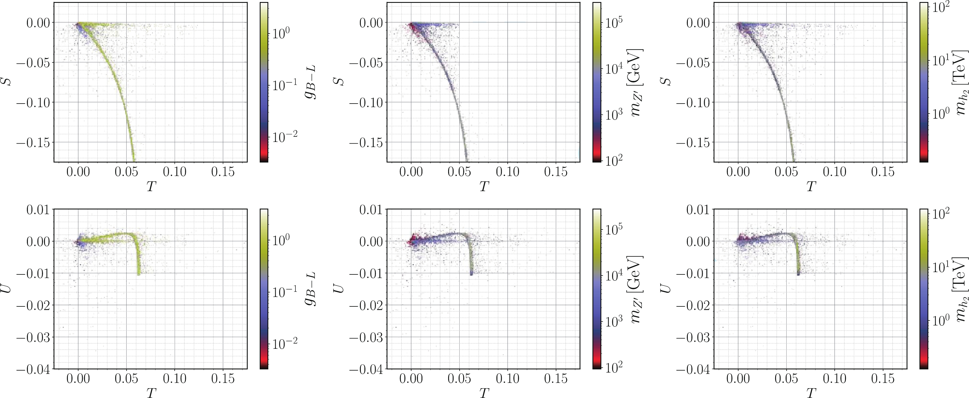

Figure 1.  (color online) Scatter plots for the EW oblique corrections in the $ST$ (upper row) and $TU$ (lower row) planes. In the color scales, their correlations with the ${U}(1)_{\rm{B - L}}$ gauge coupling $g_{\rm{B-L}}$, $Z^\prime$ mass, $m_{Z^\prime}$, and second Higgs mass, $m_{h_2}$, are shown in left, middle, and right panels, respectively. The points shown here satisfied the unitarity constraints in SPheno 4.0.3 [61, 62] as well as the Higgs phenomenology constraints in HiggsBounds 4.3.1 [68] and HiggsSignals 1.4.0 [69].

Current precision measurements [31] provide the allowed regions

where S-T are 92% correlated, while S-U and T-U are -66% and -86% anti-correlated, respectively. We compare our results with the EW fit in Eq. (31) and require consistency with the best fit point within a 95% C.L. ellipsoid (see Ref. [28] for further details about this method). We show in Fig. 2 our results in the $ST$ (upper row) and $TU$ (lower row) planes, where colored points are consistent with the EW precision observables at 95% C.L., whereas grey ones lie outside the corresponding ellipsoid of the best fit point and are thus excluded from our analysis. The color scales show correlations with the scalar quartic couplings $\lamb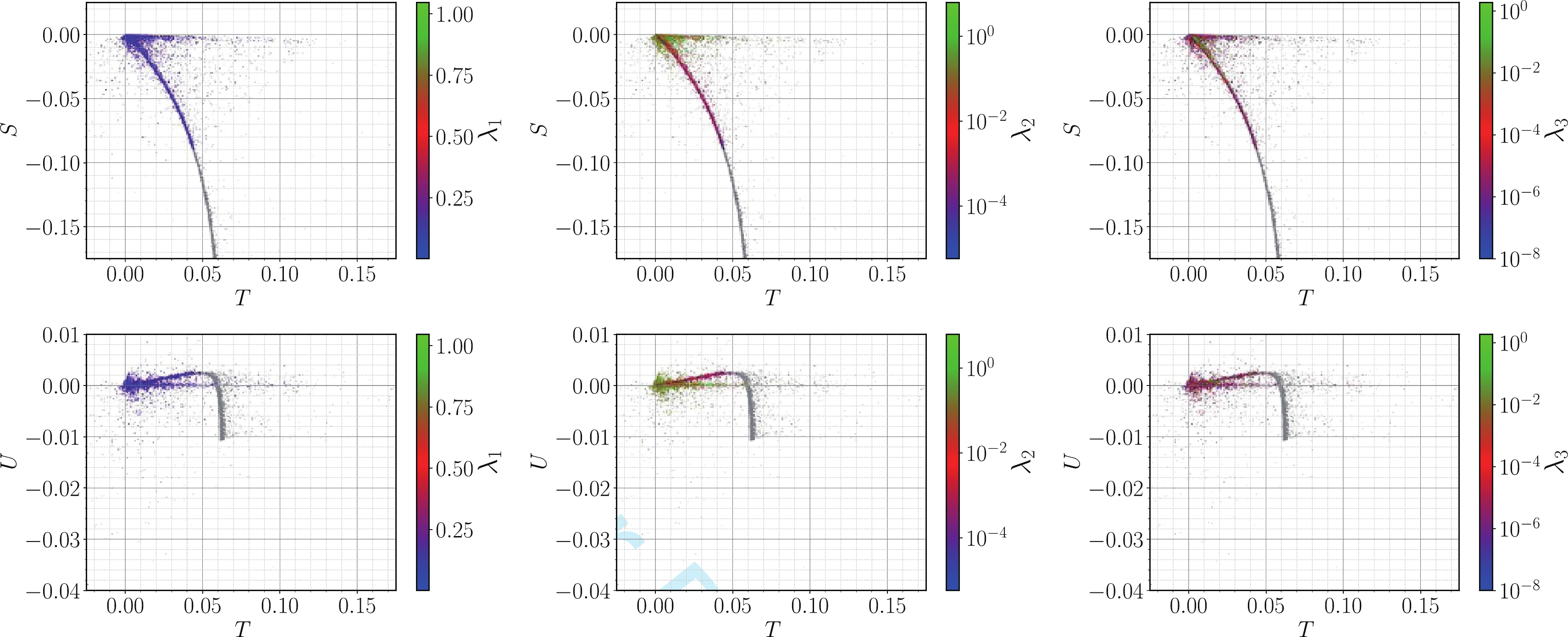da_{1,2,3}$.

Figure 2.  (color online) Scatter plots for the EW oblique corrections in the $ST$ (upper row) and $TU$ (lower row) planes versus the scalar quartic couplings $\lambda_{1,2,3}$ shown in the color scale. Accepted points lying within a 95% C.L. ellipsoid of the best fit point and hence satisfying the EW precision constraints are given in color, whereas grey points are excluded. Other constraints are the same as in Fig. 1.

The B-L-SM predicts a new visible scalar, which we denote as $h_2$, in addition to a SM-like $125\; {\rm{GeV}}$ Higgs boson, $h_1$. Thus, in a second layer of phenomenological tests in both Figs. 1 and 2, we also implemented the collider bounds on the Higgs sector. In particular, we use HiggsBounds 4.3.1 [68] to apply 95% C.L. exclusion limits to a new scalar particle, $h_2$, and HiggsSignals 1.4.0 [69] to check for consistency with the observed Higgs boson, taking into account all known Higgs signal data. For the latter, we have accepted points whose fit to the data replicates the observed signal at 95% C.L., while the measured value for its mass, $m_{h_1} = 125.10 \pm 0.14\; {\rm{GeV}}$ [31], is reproduced within a $3\sigma$ uncertainty. The required input data for HiggsBounds/HiggsSignals are generated by the SPheno output in the format of a SUSY Les Houches Accord (SLHA) [70] file. In particular, it provides scalar masses, total decay widths, Higgs decay branching ratios, and the squared SM-normalized effective Higgs couplings to fermions and bosons (that are needed for analysis of the Higgs boson production cross sections). For details about this calculation, see Ref. [68].

As the third layer of phenomenological tests, in this work, we have studied the viability of the surviving scenarios from the perspective of direct collider searches for a new $Z^\prime$ gauge boson. We have used MadGraph5_aMC@NLO 2.6.2 [71] to compute the $Z^\prime$ Drell-Yan production cross section and subsequent decay into the first- and second-generation leptons, i.e., $\sigma(pp \to Z^\prime) \times$$B(Z^\prime \to \ell \ell)$ with $\ell = e,\; \mu$, and then compared our results to the most recent ATLAS exclusion bounds from the LHC runs at the center-of-mass energy $\sqrt{s} = 13\; {\rm{TeV}}$ and integrated luminosity of 139 fb$^{-1}$ [53]. The SPheno SLHA output files were used as parameter cards for MadGraph5_aMC@NLO, where the information required to calculate $\sigma(pp \to Z^\prime) \times B(Z^\prime \to \ell \ell)$, such as the $Z^\prime$ boson mass and its total width and decay branching ratios into lepton pairs, is provided. In accordance with the experimental analysis, we have imposed a transverse momentum cut of 30 GeV for both final-state leptons while their pseudorapidities were limited to $|\eta| < 2.5$. Analogous analysis by the CMS Collaboration [54] relies on a more complicated set of kinematic variables. Thus, in the current work, for simplicity, we have only considered the ATLAS bound on $\sigma(pp \to Z^\prime) \times B(Z^\prime \to \ell \ell)$ that is sufficient for our purposes.

An important and rather restrictive constraint that needs to be taken into account results from the LEP limits on four-fermion contact interactions [72, 73]. In particular, we see from Tab. 3.13 of [72] that, for the B-L-SM, this translates into the 95% C.L. upper bounds on the $g_{\rm{{L,R}}}^{{\ell \ell Z'}}$ couplings

This also poses upper limits on the ${U}(1)_{\rm{B - L}}$ and kinetic mixing gauge couplings $g_{\rm{B - L}}$ and $g_{{\rm{YB}}}$, respectively, which are related to $g_{\rm{{L,R}}}^{{\ell \ell Z'}}$ via Eq. (35).

Let us now discuss the phenomenological properties of the B-L-SM. First, we focus on the current collider constraints and study their impact on both the scalar and gauge sectors.

We show in Fig. 3 the scenarios generated in our parameter space scan (for the input parameter ranges, see Table 3) that have satisfied all theoretical constraints, such as boundedness from below, unitarity, and EW precision tests; these scenarios are compatible with the SM Higgs data and have a new visible scalar$h_2$unconstrained by the direct collider searches. In the left panel, we show the $Z^\prime$ production cross section times its branching ratio to the first- and second-generation leptons, $\sigma B \equiv \sigma(pp \to Z^\prime) \times$$B(Z^\prime \to \ell \ell )$ with $\ell = e,\mu$, as a function of the new vector boson mass and the new physics contribution to the muon anomalous magnetic moment $\Delta a^{\rm{NP}}_\mu$ (color scale). In the right panel, we show the new scalar mass as a function of the same observables. All points above the solid line are excluded at 95% C.L. by the limit on $Z^\prime$ direct searches at the LHC performed by the ATLAS experiment [53] and are represented in grey shades. Darker shades denote would-be-scenarios with larger values of $\Delta a^{\rm{NP}}_\mu$ , while smaller contributions to this observable are represented with lighter shades. The red cross in our figures signals the lightest $Z^\prime$ found in our scan, which we regard as a possible early-discovery (or early-exclusion) benchmark point in the forthcoming LHC runs. Such a benchmark point is shown in the first line of Table 4. In the right panel, we notice that the new scalar bosons can become as light as $400\; {\rm{GeV}}$, with $Z^\prime$ masses being above $5.2\; {\rm{TeV}}$. Such a moderately large minimal value for the new Higgs boson mass results from the fact that both the $h_2$ and the $Z'$ bosons share a common VEV in their mass forms, as seen from Eqs. (13) and (27). Then, while direct searches at the LHC for a B-L-SM $Z'$ boson keep pushing its mass to larger values, the new Higgs boson mass also increases linearly with $m_{Z'}$ according to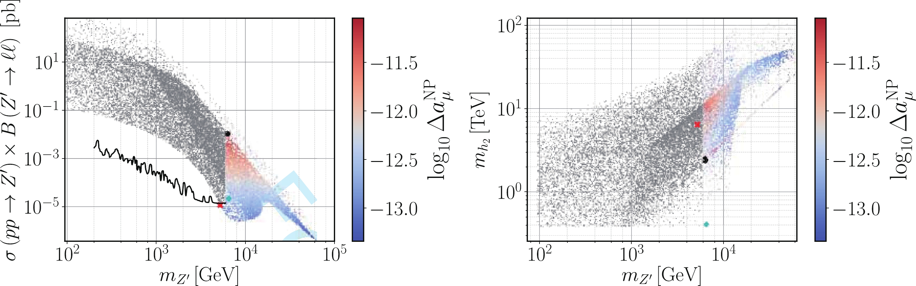

Figure 3.  (color online) Scatter plots showing the $Z^\prime$ Drell-Yan production cross section times the decay branching ratio into a pair of electrons and muons (left panel) and the new scalar mass $m_{h_2}$ (right panel) as functions of $m_{Z^\prime}$ and the new physics (NP) contributions to the muon $\Delta a_\mu$ anomaly. The solid line represents the current ATLAS expected limit on the production cross section times the branching ratio into a pair of leptons at 95% C.L., taken from Ref. [53]. Colored points have satisfied all theoretical and experimental constraints, while grey points are excluded by direct $Z^\prime$ searches at the LHC. The six highlighted points in both panels denote the benchmark scenarios described in Table 4. These are represented by the red cross for the lightest $Z^\prime$ scenario (first row), cyan diamond for the lightest $h_2$ scenario (second row), and the black dots (last four rows).

$m_{Z^\prime}$	$m_{h_2}$	x	$\log_{10} \Delta a_\mu^{\rm{NP}}$	$\sigma B$	$\theta_W^\prime$	$\log_{10}\alpha_h$	$g_{\rm{B - L}}$	$g_{{\rm{YB}}}$	$g_{{\rm{L}}}^{{\ell \ell Z^\prime}} = g_{\rm{R}}^{{\ell \ell Z^\prime}}$
$5.199$	$6.41$	$15.4$	$-13.01$	$1.16 \times 10^{-5}$	$\approx 0$	$-5.18$	$0.17$	$2.0\times 10^{-5}$	$0.08$
$6.478$	$0.41$	$9.77$	$-12.57$	$2.15 \times 10^{-5}$	$3.22\times 10^{-7}$	$-5.85$	$0.34$	$1.7\times 10^{-3}$	$0.17$
$6.371$	$2.34$	$1.08$	$-11.05$	$0.01$	$1.05\times 10^{-6}$	$-7.31$	$1.97$	$2.1\times 10^{-3}$	$0.98$
$6.260$	$2.31$	$1.15$	$-11.07$	$0.01$	$5.87\times 10^{-5}$	$-2.79$	$1.87$	$0.125$	$0.94$
$6.477$	$2.40$	$1.14$	$-11.08$	$0.01$	$2.75\times 10^{-5}$	$-4.29$	$1.93$	$0.06$	$0.97$
$6.252$	$2.53$	$1.28$	$-11.08$	$0.01$	$\approx 0$	$-8.65$	$1.86$	$1.6\times 10^{-5}$	$0.93$

Table 4.  A selection of five benchmark points represented in Figs. 3 and 6 to 8. The $m_{Z^\prime}$, $m_{h_2}$, and x parameters are given in TeV. The second line represents the point with lightest possible $h_2$, while the first one shows the lightest allowed $Z^\prime$ boson found in our scan. The last four lines show four points that yield a minimal tension of $3.28$ standard deviations, with the combined theoretical and experimental error of the muon $(g-2)_\mu$ anomaly.

Furthermore, neither $\lambda_2$ can be arbitrarily small (see Fig. 2 central panels) nor $g_{\rm{B-L} }$ can be arbitrarily large (see Fig. 1 left panels) in order to compensate an increase in $m_{Z'}$. We highlight with a cyan diamond the benchmark point with the lightest $h_2$ boson within this range. This point is shown in the second line of Table 4.

The same observation can also be made from Fig. 4 , which represents the points excluded by the Higgs physics constraints and by the ATLAS $Z'$ search constraints as well as passed physically valid points in our numerical scan. The left panel shows the the scalar VEV versus the second Higgs mass and the $Z'$ mass, while the right panel illustrates such a dependence for $\lambda_2$ coupling roughly related to $m_{h_2}$ by means of Eq. (33). Indeed, we observe that owing to the Higgs physics constraints, $\lambda_2$ cannot be arbitrarily small in order to compensate a larger $Z’$ mass (thus, a large singlet VEV). In particular, the smaller the VEV or $m_{Z’}$, the larger the $\lambda_2$. Therefore, the Higgs search imposes the strongest constraints on $m_{h_2}$, at least, in the case of a large $Z’$ mass.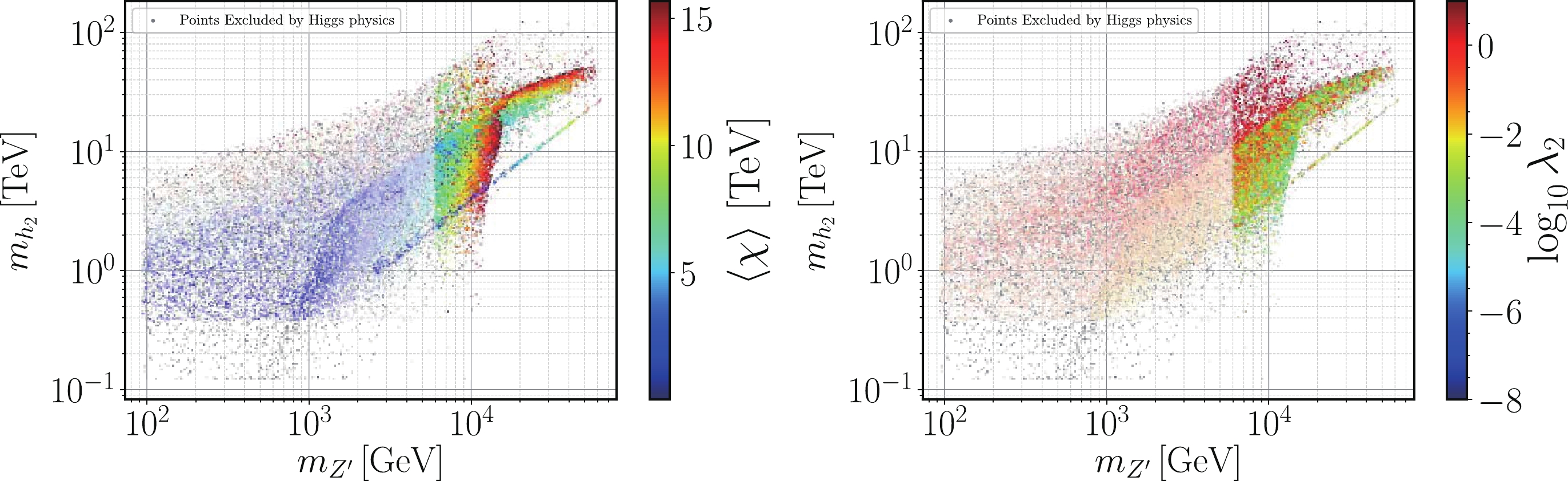

Figure 4.  (color online) Scatter plots showing the scalar VEV (left) and the $\lambda_2$ coupling (right) versus the second Higgs mass and the $Z'$ mass. All the shown points satisfy the theoretical and phenomenological constraints except the Higgs physics constraints (grey points) and ATLAS $Z'$ search constraints (faded colored points), while the colored points are the physically valid points that pass all the exclusion limits.

Looking again at Fig. 3 (left panel), we see that there is a dark-red region where $\Delta a_\mu^{\rm{NP}}$ can be enhanced up to a maximum of $\Delta a_\mu^{\rm{NP}} = 8.9 \times 10^{-12}$ for a range of $m_{Z^\prime}$ boson masses approximately between $6.3\; {\rm{TeV}}$ and $6.5\; {\rm{TeV}}$, representing a very small improvement in comparison with the SM prediction. Such a mass region is particularly interesting as it can be probed by the forthcoming LHC runs. If a $Z^\prime$ boson discovery remains elusive, it can exclude a possibility of alleviating the tension between the measured and the SM prediction for the muon $\left(g-2\right)_\mu$ anomaly in the context of the B-L-SM. However, note that, with new measurements at the E989 experiment at Fermilab, if a partial reduction in the current discrepancy is observed, the B-L-SM prediction may become an important result and a motivation for future $Z'$ searches at the LHC. Note that such maximal $\Delta a^{\rm{NP}}_\mu$ values represent a rather small region of scattered red points where the new scalar boson mass takes values of a few TeV. Furthermore, in some scenarios represented by the second and third lines in Table 4, the $\theta_W^\prime$ and $\alpha_h$ angles are not vanishingly small, which may hint about certain possibilities for observing both a new scalar and new vector boson in this region.

New physics contributions $\Delta a_\mu^{\rm{NP}}$ to the muon anomalous magnetic moment are given on the one-loop order by the Feynman diagrams depicted in Fig. 5. Since the couplings of a new scalar $h_2$ to the SM fermions are suppressed by a factor of $\sin \alpha_h$, which we find to be always smaller than $0.002$, as can be seen in the bottom panel of Fig. 6, the right diagram in Fig. 5, which scales as $\Delta a_\mu^{h_2} \propto \dfrac{m_\mu^2}{m_{h_2}^2}(y_\mu \sin \alpha_h)^2$ with $y_\mu = Y_e^{22}$, provides sub-leading contributions to $\Delta a_\mu$. Furthermore, as we show in the top-leftpanel of Fig. 6 , the new scalar boson mass, which we have found to satisfy $m_{h_2} \gtrsim 400\; {\rm{GeV}}$, is not sufficiently light to compensate the smallness of the scalar mixing angle. Conversely, recalling that all fermions in the B-L-SM transform non-trivially under ${U}(1)_{\rm{B - L}}$, the new $Z^\prime$ boson can have sizeable couplings to fermions via gauge interactions proportional to $g_{\rm{B - L}}$ and $g_{{\rm{YB}}}$, essentially constrained by four fermion contact interactions.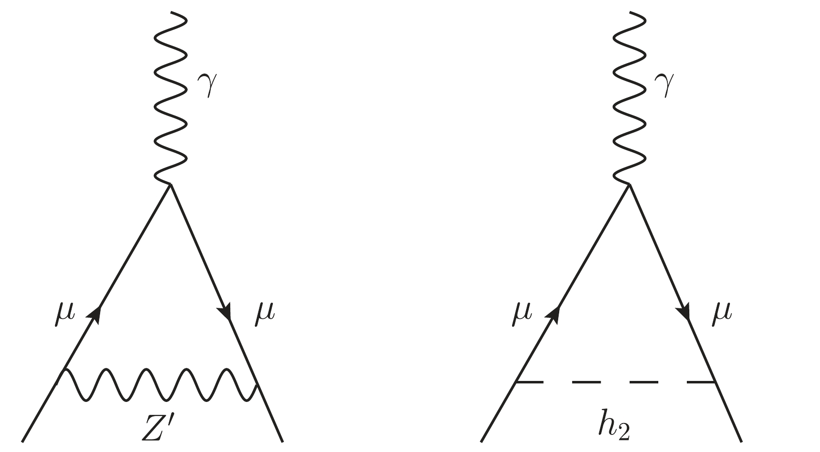

Figure 5.  One-loop diagrams contributing to $\Delta a_\mu^{\rm{NP}}$ in the B-L-SM.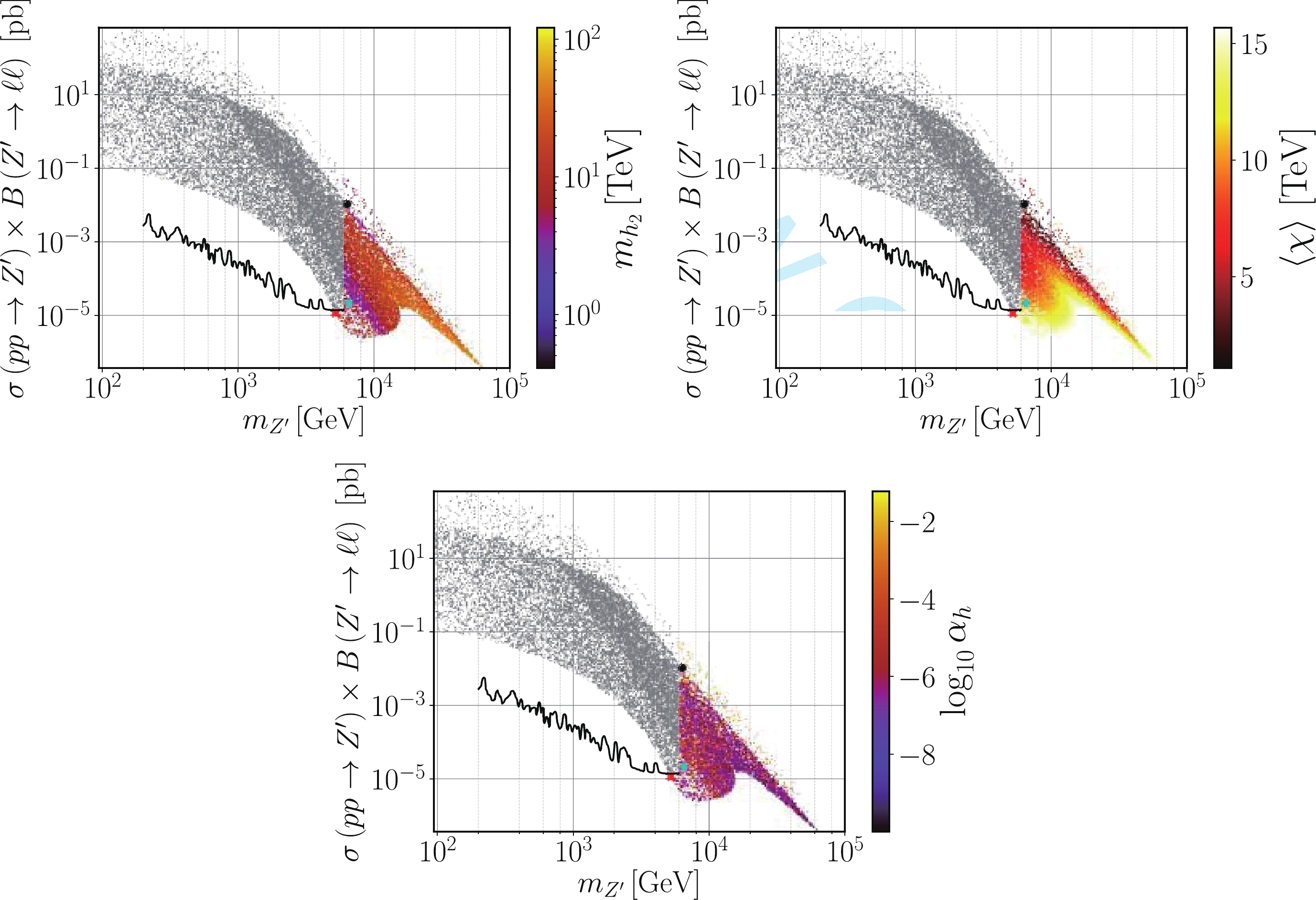

Figure 6.  (color online) Scatter plots showing the $Z^\prime$ Drell-Yan production cross section times the decay branching ratio into a pair of electrons and muons in terms of the $m_{Z^\prime}$ boson mass. The color gradation represents the new scalar mass (top-left), the ${U}(1)_{\rm{B - L}}$-breaking VEV (top-right), and the scalar mixing angle (bottom). The notation is the same as in Fig. 3 (left).

Therefore, the left diagram in Fig. 5 provides the leading contribution to $\left(g-2\right)_\mu$ in the model under consideration. In particular, $\Delta a_\mu^{Z^\prime}$ can be written as

where the left- and right-chiral projections of the charged lepton couplings to the $Z^\prime$ boson, $g_{{\rm{L}}}^{{\ell \ell Z^\prime}}$ and $g_{\rm{R}}^{{\ell \ell Z^\prime}}$, respectively, can be approximated as follows

to the second order in the $v/x$-expansion. The regions of the parameter space that we are exploring feature a heavy $Z'$ boson such that $m_\mu^2 \ll m_{Z'}^2$. In this limit, the loop functions $g_{\rm{FFV}}\left(\dfrac{m_\mu^2}{m_{Z'}^2}\right)$ and $f_{\rm{FFV}}\left(\dfrac{m_\mu^2}{m_{Z'}^2}\right)$ tend to the values $g_{\rm{FFV}}(0) \to 4$ and $f_{\rm{FFV}}(0) \to - {4}/{3}$, where Eq. (34) can be approximated as

If $v/x \ll 1$, corresponding to the lighter shades of the color scale in the top-right panel of Fig. 6, we can further approximate^①

With this, the $Z'$ contribution to the muon anomalous magnetic moment can be recast as

and for $g_{{\rm{YB}}} \ll g_{\rm{B - L}}$, which represents the majority of the points in our scan,

Note that, limits from four fermion contact interactions do not allow $g_{\rm{B - L}}$ to be sufficiently large to contribute to a sizeable $\Delta a_\mu^{\rm{NP}}$ via Eqs. (38) or (39). In particular, we found that $g_{\rm{B - L}}$ is always smaller than $1.97$ as depicted in the bottom panel of Fig. 7. In contrast, limits on the $\theta_W^\prime$ mixing angle and those from four-fermion contact interactions do not forbid an order one $g_{{\rm{YB}}}$ coupling in the sparser upper edge of the top-left panel of Fig. 7. It is indeed such a sizeable $g_{{\rm{YB}}}$ that only slightly enhances the muon $(g-2)_\mu$ anomaly, as can be seen in the red region of both plots in Fig. 3. We have found four benchmark points represented by the black dots in Figs. 3 and 6 to 8, where the tension between the current combined $1 \sigma$ error of the muon anomalous magnetic moment and the B-L-SM prediction is alleviated only by at most $0.01$ standard deviations compared with the SM, a totally negligible effect. These points are shown in the third to sixth rows of Table 4.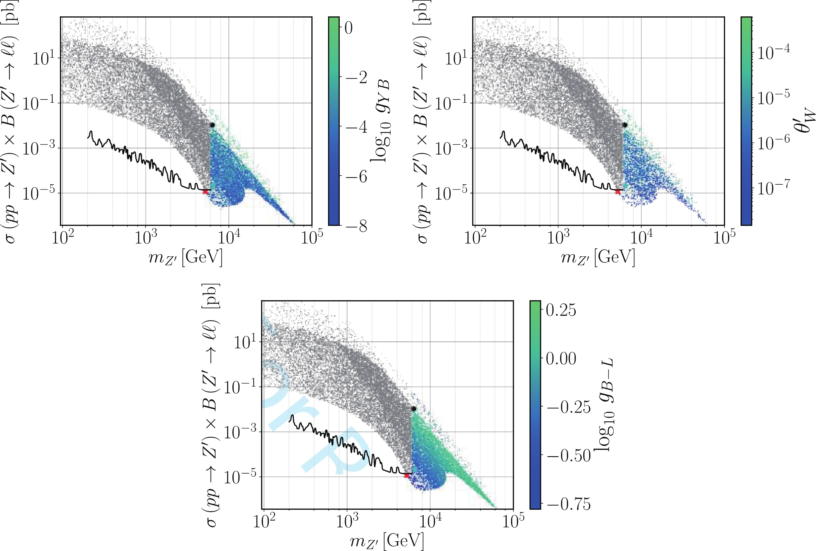

Figure 7.  (color online) The same as in Fig. 6 but with the color scale representing the gauge-mixing parameters, $g_{{\rm{YB}}}$ (top-left) and $\theta_W^\prime$ (top-right), and the ${U}(1)_{\rm{B - L}}$ gauge coupling, $g_{\rm{B - L}}$ (bott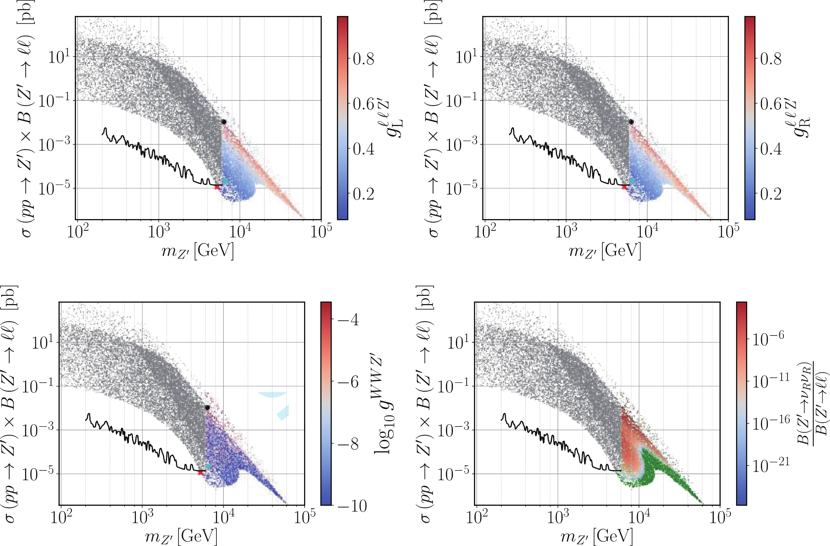om).

Figure 8.  (color online) The same as in Fig. 6 but with the color scale representing the coupling of leptons to $Z^\prime$ (top panels), the coupling of W bosons to $Z^\prime$ (bottom left), and the ratio of the $Z^\prime$ branching fraction to right-handed neutrinos $\nu_R$ over its branching fraction to charged leptons (bottom-right). In the bottom-right panel, green points correspond to allowed scenarios with fixed $B(Z^\prime \to \nu_R \nu_R) = 0$.

A close inspection of Fig. 3 (left panel) and Fig. 6 (top-right panel) reveals an almost one-to-one correspondence between the color shades. This suggests that $\Delta a_\mu^{Z^\prime}$ must somehow be related to the VEV x. To understand this behavior, let us also look at Fig. 7 (top-left panel) where we see that the coupling $g_{{\rm{YB}}}$ is typically very small apart from the green band at the upper edge, where it becomes an order of one. For the relevant parameter space regions, Eq. (27) is indeed a good approximation, as was argued above. It is then possible to eliminate $g_{\rm{B - L}}$ from Eq. (39) and rewrite it as

which explains the observed correlation between both Fig. 3 (left panel) and Fig. 6 (top-right panel). Note that this simple and illuminating relation becomes valid as a consequence of the heavy $Z^\prime$ mass regime, in combination with the smallness of the $\theta_W^\prime$ mixing angle required by the LEP constraints. Indeed, while we have not imposed any strong restriction on the input parameters of our scan (see Table 3), Eq. (23) necessarily implies that both $g_{{\rm{YB}}}$ and $v/x$ cannot be simultaneously sizeable, in agreement with what is seen in Fig. 7 (top-left panel) and Fig. 6 (top-right panel). The values of $\theta_W^\prime$ obtained in our scan are shown in the top-right panel of Fig. 7.

For completeness, we show in Fig. 8 the physical couplings of $Z^\prime$ to muons (top panels) and to $W^\pm$ bosons (bottom left panel). Note that, for the considered scenarios, the latter can be written as

While both $g_{\rm{B - L}}$ and the ratio $v/x$ provide a smooth continuous contribution in the $\sigma B - m_{Z^\prime}$ projection of the parameter space, the observed blurry region in $g^{WWZ^\prime}$ is correlated with the one in the top-left panel of Fig. 7 as expected from Eq. (41). In contrast, the couplings to leptons $g_{\rm L,R}^{\ell \ell Z^\prime}$ exhibit a strong correlation with $g_{\rm{B - L}}$ in Fig. 7 except for the sparser region at the upper edge of the $\sigma B - m_{Z^\prime}$ plane where the correlation becomes proportional to $g_{{\rm{YB}}}$, in agreement with our discussion above and with Eq. (37). In the bottom-right panel of Fig. 8, we also show the relative value of the $Z^\prime$ branching ratio into a pair of right-handed neutrinos, $B(Z^\prime \to \nu_R \nu_R)$, versus the corresponding branching fraction into charged leptons. We have found that the $Z^\prime$ decay into right-handed neutrinos is strongly suppressed for all the points that satisfy the theoretical and experimental constraints and thus cannot significantly impact the exclusion bounds.

To conclude our analysis, one should note that the two-loop Barr-Zee type diagrams [74] are always subdominant in our case. To see this, let us consider the four diagrams shown in Fig. 9. The same reason that suppresses the one-loop $h_2$ contribution in Fig. 5 is also responsible for the suppression of both the top-right and bottom-right diagrams in Fig. 9 (for details see Ref. [75]). Recall that the coupling of $h_2$ to the SM particles is proportional to the scalar mixing angle $\alpha_h$, which is always small (or very small), as we can see in Fig. 6. An analogous effect is present in the diagram involving a W-loop, where a vertex proportional to $g^{WWZ^\prime}$ suppresses such a contribution. The only diagram that might play a sizeable role is the top-left one, where the couplings of $Z^\prime$ to both muons and top quarks are not negligible.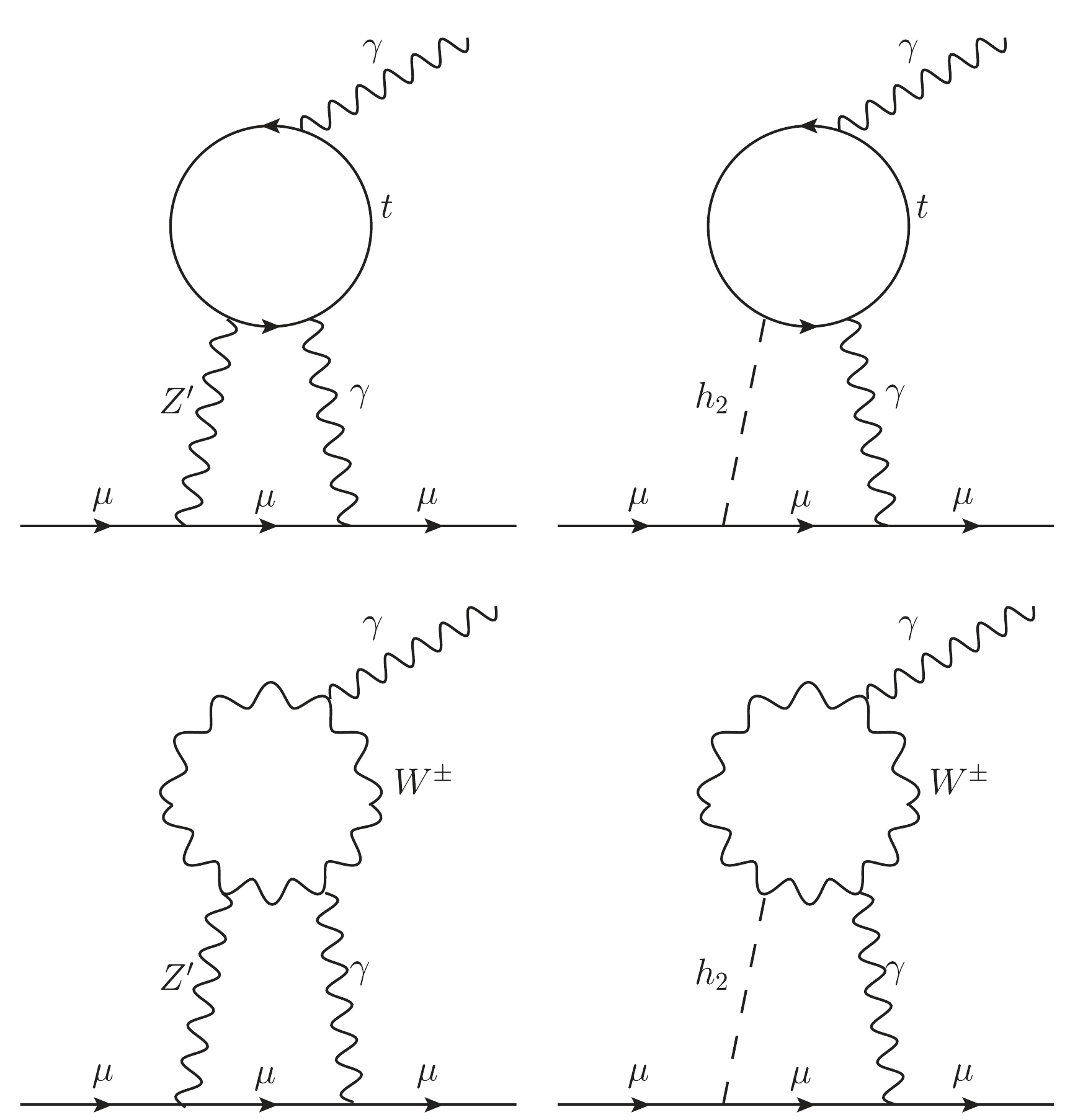

Figure 9.  Barr-Zee type two-loop diagrams contributing to $\Delta a_\mu$.

Let us then estimate the size of the first diagram in Fig. 9. Diagrams of this type were already presented in Ref. [76] but for the case of a SM Z-boson. Since the same topology also holds for the considered case of the B-L-SM, if we substitute Z with the new $Z^\prime$ boson, the contribution to the muon $(g-2)_\mu$ anomaly can be rewritten as

where $g_{\rm L, R}^{ttZ^\prime}$, calculated in SARAH, are the left- and right-chirality projections of the $Z^\prime$ coupling to top quarks, given by

The loop integral ${\rm{T}}_7 (m_{Z^\prime}^2, m_t^2, m_t^2)$ was determined in Ref. [76] and, in the limit $m_{Z^\prime} \gg m_t$, as we show in Eq. (54), it is simplified to

up to a small truncation error (see Appendix A for details). For the parameter space region under consideration, the difference $g_{\rm{L}}^{ttZ^\prime} - g_{\rm{R}}^{ttZ^\prime}$ can be cast in a simplified form as follows

Using this result and the approximate value of the loop factor, we can calculate the ratio between the Barr-Zee type and one-loop contributions to the muon $(g-2)_{\mu}$,

which shows that $\Delta a_\mu^{\gamma Z^\prime}$ does indeed play a subdominant role in our analysis and can be safely neglected.

To summarize, in this work, we have performed a detailed phenomenological analysis of the minimal ${\rm{U}}(1)_{\rm{B - L}}$ extension of the Standard Model known as the B-L-SM. In particular, we have confronted the model with the most recent experimental bounds from the direct $Z^\prime$ boson and next-to-lightest Higgs state searches at the LHC, as well as with the LEP constraints on four-fermion contact interactions. Simultaneously, we have analyzed the prospects of the B-L-SM for a better explanation of the observed anomaly in the muon anomalous magnetic moment $(g-2)_{\mu}$ in comparison with the SM. For this purpose, we have explored the B-L-SM potential for interpretation of the $(g-2)_{\mu}$ anomaly in the regions of the model parameter space that are consistent with current constrains from the direct searches and electroweak precision observables.

We have studied the correlations of the $Z^\prime$ production cross section times the branching ratio into a pair of light leptons versus the physical parameters of the model. In particular, we have found that the muon $(g-2)_{\mu}$ observable dominated by $Z^\prime$ loop contributions is maximized for $m_{Z^\prime}$ between $6.3$ and $6.5\; {\rm{TeV}}$. As one of the main results of our analysis, we have found phenomenologically consistent model parameter space regions that simultaneously fit the exclusion limits from direct $Z^\prime$ searches and maximize the muon $(g-2)_\mu$ contribution to a value of $8.9 \times 10^{-12}$. This represents a marginal or no improvement in comparison with the SM prediction. The new Muon $(g-2)_\mu$ E989 experiment at the Fermilab will be able to measure this anomaly with an increased precision of $0.14\; {\rm{ppm}}$. If a larger new physics contribution to this observable is confirmed, the B-L-SM can not be considered as a candidate theory to explain that effect.

One should notice here that the recent lattice result by the BMW collaboration [77] suggests that there is no need for new physics to explain the muon $(g-2)_\mu$ data. If correct, this eliminates the necessarily large effects in the muon $(g-2)_\mu$ coming from the B-L-SM, compared with the SM. While a confirmation of the currently observed anomaly with a smaller error can become rather exciting news, a more pessimistic scenario when the discrepancy either disappears or partially reduces, would reinforce the significance of our result and offer a motivation for future $Z'$ searches at the LHC in the $5-7\; {\rm TeV}$ domain. Along these lines, we have identified five benchmark points for future phenomenological explorations: one scenario with the lightest $Z^\prime$ ($m_{Z^\prime}\simeq 5.2$ TeV), another scenario with the lightest second scalar boson ($m_{h_2}\simeq 400$ GeV), and three other scenarios that maximize the muon $(g-2)_{\mu}$ anomaly. Another important result resides in the fact that an increasingly heavy $Z'$ boson also pushes up the mass of the second Higgs boson. Therefore, the hypothetical observation of such a new physics state as a scalar or a vector boson would pose stringent constraints on the B-L-SM. For completeness, we have also estimated the dominant contribution from the Barr-Zee type two-loop corrections and found a relatively small effect.

To finalize, let us comment that with all most relevant constraints incorporated in our numerical analysis, while the best explanation of the muon $(g-2)_\mu$ in the B-L-SM predicting a value marginally above the SM one is not satisfactory, our result offers an important piece of information that can be relevant for the upcoming $a_\mu$ precision measurements at Fermilab as well as for building less minimal models containing heavy $Z'$ bosons and capable of a good explanation of the muon $(g-2)_\mu$ anomaly. Another research direction that can be pursued is the BL-SM analysis for the conditions of the HL-LHC. Along these lines, a significance calculation in future $Z’$ searches, similar to the one performed very recently in the 3-3-1 model in Ref. [78] that is probing the $Z’$ boson mass up to 4 TeV at the HL-LHC, should be pursued aiming at probing vast regions of the parameter space still allowed by the LHC searches.

The authors would like to thank Werner Porod and Florian Staub for discussions on the SPheno implementation of the muon $(g-2)_{\mu}$. The authors would also like to thank Nuno Castro, Maria Ramos and Emanuel Gouveia for insightful discussions about the implementation of the current model in MadGraph5_aMC@NLO. J.P.R thanks Lund University for hospitality during a short and fruitful visit.

In Appendix B of Ref. [76], the exact integral equations for ${\rm{T}}_7(x,y,z)$ are provided. In our analysis, we consider the limit where $x \gg y = z$, with $x = m_{Z^\prime}^2$ and $y = z = m_t^2$; Eq. (44) provides a good approximation up to a truncation error. Here, we show the main steps in determining Eq. (44). The exact form of the loop integral reads

with $\varphi_0 (x,y)$ and $\Phi(x,y,z)$ defined in Ref. [76]. Let us now expand each of the terms for $x \ll y$. While the first term is exact and has the form

the second can be approximated as

In Eq. (49), the $\xi = {1}/{3}$ factor was introduced in order to compensate for a truncation error. This was obtained by comparing the numerical values of the exact expression and our approximation. The third term can be simplified to

and the fourth to

The fifth and the seventh terms read

and finally, the sixth term can be expanded as

Noting that Eq. (48) is of the order ${1}/{x^2}$, combining Eqs. (47), (49), (50), (51), (52), and (53), we get the following for the leading ${1}/{x}$ contributions: