Gluon-pair-creation production model of strong interaction vertices

According to the theory of the strong interaction, quantum chromodynamics (QCD) [1], gluons are able to interact with one another, which suggests the existence of a particle consisting solely of gluons, the glueball. The search for the glueball has a long history, however evidence of its existence is still vague. Being short of reliable glueball production and decay mechanisms makes the corresponding investigation rather difficult. Another hurdle hindering the search for the glueball lies in the fact that they usually mix heavily with the quark states, somehow with the exception of exotic glueballs [2].

Scalar glueballs which have the quantum numbers $J^{PC} = 0^{++}$ are suggested to be the lightest glueballs by lattice calculation, displaying a mass of around $1600-1700$ MeV with an uncertainty of about $100$ MeV [3-6]. Experimentally, there exist three isosinglet scalars that exist in this mass range: $f_0(1370)$, $f_0(1500)$ , and $f_0(1710)$. The absence of the $\gamma\gamma\to K\bar{K}$ or $\pi^+\pi^-$ pair production modes through $f_0(1500)$ excludes the possibility of a large $n\bar{n}$ content within $f_0(1500)$ [7, 8]. On the other hand, the $f_0(1500)$ has a small $K\bar{K}$ decay branching rate [9-12], implying that its main content is unlikely to be $s\bar{s}$. Various peculiar natures suggest that $f_0(1500)$ might be a scalar glueball or a glue rich object [13]. In a large mixing model, as discussed in Refs. [13-16], glue is shared between $f_0(1370)$, $f_0(1500)$ , and $f_0(1710)$. The isosinglet scalar $f_0(1370)$ is mainly constructed of $n\bar{n}$, $f_0(1500)$ is thought to be glue predominant, and $f_0(1710)$ has a high $s\bar{s}$ content.

Evidence for pseudoscalar $0^{-+}$ glueballs is still weak [17]. $E(1420)$ and $\iota(1440)$ observed by Mark II were early candidates of pseudoscalar glueballs [18-21]. However, $E(1420)$ was later considered to be $1^+$ meson and renamed $f_1(1420)$, while $\iota(1440)$ is still thought to be a pseudoscalar, now known as $\eta(1405)$ [22]. The mode $\eta(1405)\to\eta\pi\pi$ was observed at BES II in $J/\psi$ decay [23] and was confirmed in $\bar{p}p$ annihilation [24]. It should be noted that $\eta(1405)$ was observed in neither $\eta\pi\pi$ nor $K\bar{K}\pi$ channels in $\gamma\gamma$ collisions by L3 [25]; this implies that $\eta(1405)$ has a large glue component since glueball production is suppressed in $\gamma\gamma$ collisions. It is also worth mentioning that the quenched lattice and QCD sum rule calculation predict that the $0^{-+}$ glueball mass might be above $2$ GeV [4, 26, 27], though Gabadadze argued that the pseudoscalar glueball mass in full QCD could be much less than the quenched lattice result in Yang-Mills theory [28]. Furthermore, despite $\eta(1405)$ fitting well with the fluxtube model [29] and roughly fitting with the $\eta$-$\eta'$-G mixing calculations [30], a recent triangle singularity mechanism analysis reveals that $\eta(1405)$ and $\eta(1475)$ might be the same state [31]. For further properties of pseudoscalar glueballs, readers may refer to recent studies [32, 33].

In this paper, motivated by studying the glueball production and decay mechanisms, we discuss glueball production in $\eta_c$ decay by introducing a model for the gluon-pair-vacuum interaction vertices; namely the $0^{++}$ model, as shown in Fig. 1. We assume the gluon pair is created homogeneously in space with equal probability. Comparing to the $^3P_0$ model [34-43], which models quark-antiquark pair creation in a vacuum, we formulate an explicit vacuum gluon-pair transition matrix and estimate the strength of the gluon-pair creation. Employing the $0^{++}$ model, we then investigate the $\eta_c$ and $\eta_b$ decays to scalar and pseudoscalar glueballs. Based on previous glueball studies, we take $f_0(1710)$ and $f_0(1500)$ as scalar glueball candidates, and $\eta(1405)$ as a pseudoscalar glueball candidate. The corresponding decay widths and branching fractions are calculated.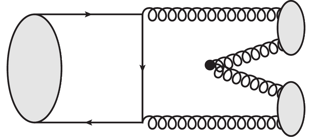

Figure 1.  Schematic diagram for glueball production in $\eta_c$ decay using the $0^{++}$ model.

The rest of the paper is arranged as follows. After the introduction, we construct a model for gluon-pair-vacuum interaction vertices in Sec. 2. The partial widths of $\eta_c \to f_0(1500)\eta(1405)$, $\eta_b\to f_0(1500)\eta(1405)$ and $\eta_b\to f_0(1710)\eta(1405)$ are evaluated in Sec. 3. Last section is remained for summary and outlooks.

In quantum field theory, the physical vacuum is thought of as the ground state of energy, with constant particle field fluctuations. Therefore, there are certain probabilities for quark pairs and gluon pairs with vacuum quantum numbers to appear in the vacuum. It is reasonable to hypothesize that gluon pairs would be created with equal amplitude in space, akin to the quark-antiquark pairs in the $^3P_0$ model. As they are created from the vacuum, the gluon pairs possess the quantum numbers $J^{PC} = 0^{++}$.

We may argue the soundness of the $0^{++}$ scheme like this: in the language of Feynman diagram, the dominant contribution to the vacuum-gluon-pair coupling may stem from the processes where two additional gluons are produced from either a parent meson or the first two gluons. It should be noted that although by naive order counting of the strong coupling, one may presumably say these processes are dominant, in fact the nonperturbative effect may impair this analysis. The most straightforward way to configure the vacuum-gluon-pair coupling is to attribute various contributions to an effective constant, analogous to the $^3P_0$ model. This is somewhat similar to the case of hadron production, where only limited hadron production processes have been proved to be factorizable, while all other processes are usually evaluated via assumptions or models.

In the remainder of our study, we investigate glueball pair production in pseudoscalar quarkonium decay using the ${0}^{++}$ model. The transition amplitude of $\eta_c$ exclusive decay to double glueballs for instance, as shown in Fig. 1, can be formulated as

Here, $G_1$ and $G_2$ represent glueballs, while $\gamma_g$ denotes the strength of gluon pair creation in the vacuum, which in principle can be extracted by fitting to the experimental data. The ${G_{\rho\sigma}^c G^{c\rho\sigma}}$ term creates the gluon pair in the vacuum. $T_2$ is the transition operator for $\eta_c$ annihilating to two gluons. The state $|\eta_c\rangle$ and $T_2$ can be expressed as

Here, ${{\bf{k}}}_c$ and ${{\bf{k}}}_{\bar{c}}$ represent the $3$-momenta of quarks c and $\bar{c}$; $\psi_{n_{\eta_c} L_{\eta_c} M_{L_{\eta_c}}} \left({\bf{k}}_c, {\bf{k}}_{\bar{c}}\right)$ is the spatial wavefunction with n, L, S, and J the principal quantum number, orbital angular momentum, total spin and the total angular momentum of $|\eta_c \rangle$, respectively; $\chi^{c \bar{c}}$ is the corresponding spin state; $\langle L_G M_{L_G} S_G M_{S_G} | J_G M_{J_G} \rangle$ is the Clebsch-Gordan (C-G) coefficient; $g_s$ denotes the strong coupling constant; $c_i$, $A^\mu_a$ and $t^a$ respectively represent the quark fields, gluon fields and Gell-Mann matrices.

Inserting the completeness relation $\sum_{G}| G \rangle\langle G | = 2E_G$ into Eq. (1), we get

where $| G \rangle$ is the shorthand notation for gluons $g_1$ and $g_2$ emitted from $\eta_c$ and the phase space integration is implied, as given in Eq. (8). $T_1$represents the operator responsible for the $G\to G_1 G_2$ transition.

Noticing that the evaluation of the gluon-pair-vacuum interaction from first principles (QCD) is currently beyond our capability, we assume the interaction vertex shown in Fig. 2 can be modeled phenomenologically, in such a way that the transition matrix $T_1$ decomposes to: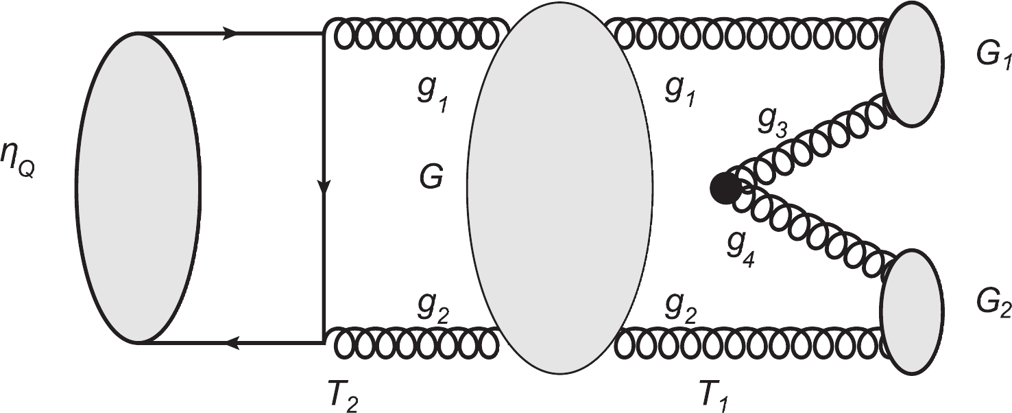

Figure 2.  The schematic Feynman diagram of a pseudoscalar quarkonium transition to a glueball pair.

where $T_{\rm vac}$ signifies the vacuum-gluon pair transition operator, and $I_i$ are identity matrices indicating the quasi-free propagations of $g_1$ and $g_2$. The gluons $g_3$ and $g_4$ are created in the vacuum, with their spin states $|m_{s_3},m_{s_4} \rangle$ having two different combinations. Please note that the gluons in the transition matrix $T_1$ turn out to be massive, after experiencing nonperturbative evolutions.

The total spin state of the gluon pair produced in the vacuum, $|S,M_S \rangle$, possessing the vacuum quantum number, being a singlet, can be formulated as

Subsequently, ${T}_{\rm vac}$ can then be expressed as

Here, ${{\bf{k}}}_3$ and ${{\bf{k}}}_4$ represent the $3$-momenta of the gluons $g_3$ and $g_4$ respectively, $a^\dagger_{3c}$ and $a^\dagger_{4d}$ are creation operators of gluons with color indices, and ${\cal{Y}}_{\ell m}({\bf{k}})\equiv |{\bf{k}}|^{\ell}Y_{\ell m}(\theta_{k},\phi_{k})$ is the $\ell$th solid harmonic polynomial that gives out the momentum-space distribution of the produced gluon pairs.

The state $| G \rangle$ should possess the quantum numbers of $| \eta_c\rangle$, i.e. $J^{PC}_G = 0^{-+}$. As discussed in previous studies [44-47], the state might mix with $\eta_c$, and thus can be parameterized as

where ${{\bf{k}}}_1$ and ${{\bf{k}}}_2$ represent the $3$-momenta of the gluons $g_1$ and $g_2$, $\psi_{n_G L_G M_{L_G}} \left({\bf{k}}_1, {\bf{k}}_2\right)$ is the spatial wavefunction with n, L, S, J the principal quantum number, orbital angular momentum, total spin and the total angular momentum of $|G \rangle$, respectively. $\chi^{1 2}$ is the corresponding spin state, later on expressed as $|S_G M_{S_G} \rangle$ for the sake of calculation transparency. $\langle L_G M_{L_G} S_G M_{S_G} | J_G M_{J_G} \rangle$ is the C-G coefficient and reads $\langle 1m;1-m | 00 \rangle$ for the state $|G \rangle$. The associated normalization conditions are

with ${{\bf{K}}_G}$ and ${{\bf{K}}'_G}$ the corresponding $3$-momenta. We have similar expressions for the $G_1$ and $G_2$ states.

Equipped with the gluon-to-glueball transition operator $T_1$ and expressions for the initial and final states, we are now capable of evaluating the transition matrix element:

Here, the momentum space integral $I_{M_{L_G},M_{L_{G_1}},M_{L_{G_2}}}({{\bf{K}}})$ can be written as

For simplicity, it is reasonable to assume that the glueball and $|G\rangle$ state wavefunctions to be in a harmonic oscillator (HO) form;

where ${\bf{k}}$ is the relative momentum between two gluons inside the states, ${\cal{N}}_{nL}$ is the normalization coefficient and ${\cal{P}}({\bf{k}}^2)$ is a polynomial of ${\bf{k}}^2$ [38]. $\langle\chi^{1 3}_{S_{G_1} M_{S_{G_1}}}\chi^{2 4}_{S_{G_2} M_{S_{G_2}}} |\chi^{1 2}_{S_G M_{S_G}} \chi^{3 4}_{00} \rangle$ which represents the spin coupling can be expressed using Wigner's $9j$ symbol [36]

Here, $s_i$ is the spin of the gluon $g_i$, with $i = 1, 2, 3, 4$, and $\sum_{S,M_s}|SM_s \rangle \langle SM_s|$ is the completeness relation.

The helicity amplitude ${\cal{M}}^{M_{J_G}M_{J_{G_1}}M_{J_{G_2}}}$ may be read off from

allowing the $\eta_c\to G_1G_2$ decay width to be readily obtained [38]:

Here, ${\cal{M}}^{J L} = \dfrac{{\cal{M}}_1^{J L} {\cal{M}}_2}{2 E_G}$, ${\cal{M}}_2$ is the amplitude of the $\eta_c \to g g$ reaction, and ${\cal{M}}_1^{J L}$ is the partial wave amplitude, obtainable from the helicity amplitude ${\cal{M}}_1^{M_{J_G}M_{J_{G_1}}M_{J_{G_2}}}$ via the Jacob-Wick formula [48], i.e.

with $J = J_{G_1}+J_{G_2}$ and $L = J_{G}-J$.

In this section, we estimate the scalar and the pseudoscalar glueball production in $\eta_c$ and $\eta_b$ decays via the $0^{++}$ model, by taking scalars $f_0(1710)$ and $f_0(1500)$, and pseudoscalar $\eta(1405)$ as the corresponding candidates, namely $G_1$ and $G_2$ respectively. The quantum numbers of the states involved in these processes are presented in Table 1; $|G\rangle$ and $|\eta_Q\rangle$ have the same quantum numbers.

	$J^{PC}$	L	$M_L$	S	$M_S$
$\eta_Q$	$0^{-+}$	$1$	$M_0$	$1$	$-M_0$
$G_1$	$0^{++}$	$0$	$0$	$0$	$0$
$G_2$	$0^{-+}$	$1$	$M_2$	$1$	$-M_2$

Table 1.  Quantum numbers of $\eta_Q$, $G_1$, and $G_2$. The values of $M_0$ and $M_2$ can be $-1$, $0$, and $1$.

In Eq. (12), the color contraction is equal to eight, and for scalar glueballs, the spin and orbital angular momentum coupling causes the C-G coefficient to be $\langle 00;00| 00\rangle = 1$. Therefore, from these results, Eq. (12) can be rewritten as

The spin coupling term $\langle\chi^{1 3}_{0 0}\chi^{2 4}_{1 -M_2} | \chi^{1 2}_{1 -M_0} \chi^{3 4}_{0 0} \rangle$ is characterized by the Wigner's $9j$ symbol, a representation of $4$-particle spin coupling, which can be expanded as series of $2$-particle spin couplings represented by Wigner's $3j$ symbols [36], shown in Appendix A.

By substituting the spin couplings provided in Appendix A into Eq. (19), we can then reduce the $T_1$ matrix element,

With a lengthy calculation (some details are given in Appendix B) the momentum space integrals are obtained, of which $I_{1,0,1} = I_{-1,0,-1} = 0$, and $I_{0,0,0}$ is given by Eq. (B8). Writing $\delta^3({\bf{K}}_G-{\bf{K}}_{G_1}-{\bf{K}}_{G_2})I \equiv I_{0,0,0}$ and considering Eqs. (16), (20) and (B8), we have

from which ${\cal{M}}_1^{M_{J_G}M_{J_{G_1}}M_{J_{G_2}}} = {\cal{M}}_1^{000}$ can be extracted out, i.e.

The probable radius R of the HO wavefunction is estimated by the relation $R = 1/\alpha$, with $\alpha = \sqrt{\mu \omega /\hbar}$. Here, $\mu$ denotes the reduced mass, $\omega$ is the angular frequency of the HO satisfying $M = (2n+L+3/2)\hbar\omega$, with M being the glueball mass, n the radial quantum number, and L the orbital angular momentum. As discussed in Refs. [49, 50], the effective mass of the constituent gluon is about $0.6$ GeV, which means $\mu \sim 0.3$ GeV for glueballs. In the calculation, the inputs we adopt are: $M_{\eta_c} = 2.98$ GeV, $M_{\eta_b} = 9.40$ GeV, $M_{f_0(1500)} = 1.50$ GeV, $M_{f_0(1710)} = 1.71$ GeV and $M_{\eta(1405)} = 1.41$ GeV [51]. Therefore, using the equations above, we can calculate the corresponding radii:$R_{\eta_c} = 2.24\;{\rm{GeV}}^{-1}$, $R_{\eta_b} = 1.26\;{\rm{GeV}}^{-1}$, $R_{f_0(1500)} = 2.79 {\rm{GeV}}^{-1}$, $R_{f_0(1710)} = 2.61\;{\rm{GeV}}^{-1}$ and $R_{\eta(1405)} = 3.26\;{\rm{GeV}}^{-1}$.

With above discussion and inputs, we can readily get I and ${\cal{M}}_1^{000}$. Please note that, when

${\cal{M}}_1^{0 0}$ can be obtained according to Eq. (18), as shown in Table 2.

	I $({\rm{GeV}})^{-3/2}$	${\cal{M}}_1^{0 0}$
$\eta_c\to f_0(1500)\eta(1405)$	$0.409$	$-0.166\gamma_g$
$\eta_b\to f_0(1500)\eta(1405)$	$-0.398$	$0.901\gamma_g$
$\eta_b\to f_0(1710)\eta(1405)$	$-0.396$	$0.897\gamma_g$

Table 2.  The I and ${\cal{M}}_1^{0 0}$ values for different processes.

The calculation of the process $\eta_Q \to gg$ is quite straightforward. At the leading order of perturbative QCD, there are only two types of decay paths, represented using Feynman diagrams in Fig. 3. Their decay amplitudes can be written as: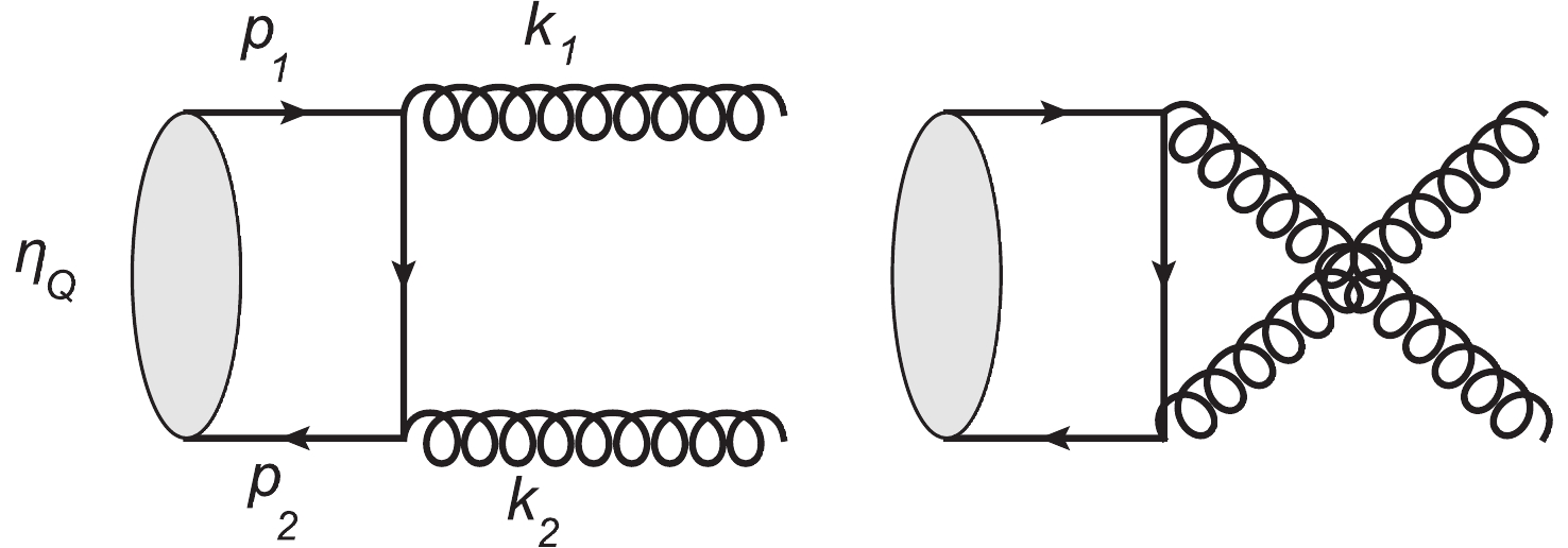

Figure 3.  The Feynman diagrams of the $\eta_Q \to gg$ decay process.

where u and $\bar{v}$ stand for heavy quark spinors, $\epsilon_\mu$ denotes the gluon polarization, and $g_s$ is the strong coupling constant. For a quark pair to form a pseudoscalar quarkonium, one can realize it by performing the following projection [52]:

Here, $m_Q$ is the heavy quark mass, $R_{\eta_Q}(0)$ denotes the radial wavefunction at the origin, and in a $\eta_Q$ center-of-mass system $p_1 = p_2\equiv p$. The $\eta_Q \to gg$ matrix element squared may be obtained through a straightforward calculation, i.e.

We estimate the strength of gluon-pair-vacuum coupling analogously to the $^3P_0$ model, where the strength of quark pair creation in vacuum is represented by $\gamma_q$ with dimensions of energy [40]. To avoid constructing a new model to mimic the nonperturbative process of the gluon pair production in the vacuum, we simply infer $\gamma_g$ by comparing the relative strength of processes $q\bar{q}\to gg$ and $q\bar{q} \to q\bar{q}$, as shown in Fig. 4. The value $\gamma_g^2/\gamma_q^2$ is assumed to be the same order of magnitude as the relative interaction rate of these two processes.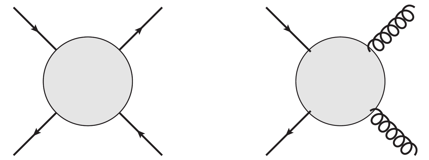

Figure 4.  The coupling of $q\bar{q}q\bar{q}$ and $q\bar{q}gg$.

It is well known that at the tree level

Considering the relationship between Mandelstam variables, we find that

where the interaction energy is set to be $\mu_{\eta_c}$, the reduced mass of the quark$-$antiquark in the decaying meson. In the $^3P_0$ model, $\gamma_q (\mu_{\eta_c}) = 0.299\times 2 m_q \sqrt{96\pi}$ [40] with $m_q = 220$ MeV [39] the value of the light quark constituent mass. Hence we find that $\gamma_g^2(\mu_{\eta_c}) \approx (5.74\pm1.93)\times 10^{-2}\ {\rm{GeV}}^{2}$. By the same method, we obtain $\gamma_g^2(\mu_{\eta_b}) \approx (2.57\pm0.86)\times 10^{-3}\ {\rm{GeV}}^{2}$.

Using Eq. (4) and the relation ${\cal{M}}^{J L} = \dfrac{{\cal{M}}_1^{J L} {\cal{M}}_2}{2 E_G}$, we find that ${\cal{M}}^{J L}$ has only one nonzero matrix element, ${\cal{M}}_1^{00} = -\dfrac{\gamma_g}{18}I\sqrt{8 E_G E_{G_1} E_{G_2}}$, and that $|{\cal{M}}_2|^2 = \dfrac{4 g_s^4 |R(0)_{\eta_Q}|^2}{3 \pi m_Q}$. Substituting these values into Eq. (17), we can then calculate the decay width of $\eta_c \to f_0(1500) \eta(1405)$,

In the above calculation, we set the charm quark mass to be $m_c = (1.27 \pm 0.03)\ {\rm{GeV}}$ [51], strong coupling constant to be $\alpha_s(\eta_c) = 0.25$, and the $\eta_c$ radial wavefunction at the origin squared to be $|R(0)_{\eta_c}|^2 = 0.527\pm0.013$ ${\rm{GeV}}^{3}$ [52]. The branching fraction of the $\eta_c \to f_0(1500)\eta(1405)$ process is then

Analogous to the $\eta_c$ decay, the $\eta_b$ exclusive decay to glueball pairs can similarly be evaluated by the $0^{++}$ model. We notice that $f_0(1710)$ is glue rich [12, 53, 54], and evaluate the process $\eta_b\to f_0(1710)\eta(1405)$ as well. Using the same procedure as for $\eta_c$, we have

For these calculations, we took the bottom quark mass to be $m_b = (4.18 \pm 0.03)\ {\rm{GeV}}$ [51], the strong coupling constant to be $\alpha_s(\eta_b) = 0.18$, and the $\eta_b$ radial wavefunction at the origin squared to be $|R(0)_{\eta_b}|^2 = 4.89\pm0.07$ ${\rm{GeV}}^{3}$ [52]. It is worthwhile to mention that although there are mixings among the $f_0(1370)$, $f_0(1500)$ and $f_0(1710)$ states [12], they do not have significant influence on our calculation results.

Moreover, from lattice QCD calculations [3-6, 26], we know that there might be scalar and pseudoscalar glueball candidates with masses of $1.75$ GeV and $2.39$ GeV, respectively. For these potential glueball candidates, we can readily calculate the branching fraction

In this work, we analyzed the processes of exclusive glueball pair production in quarkonium decays by introducing a $0^{++}$ model. This model was employed to phenomenologically mimic the gluon-pair-vacuum interaction vertices and is applicable to studies of glueball and hybrid state production. It was assumed that a gluon pair is created homogeneously in space with equal probability. By virtue of the $^3P_0$ model, we formulated an explicit vacuum gluon-pair transition matrix and estimated the strength of the gluon-pair creation. We subsequently applied this method and the results for the calculation of the $\eta_c$ to $f_0(1500)$ $\eta(1405)$ decay process, where $f_0(1500)$ and $\eta(1405)$ are respective scalar and pseudoscalar glueball candidates. We found that the decay width and branching fraction of this decay process are ${27.41}$ keV and ${8.62\times 10^{-3}}$ respectively.

In light of the $\eta_c$ decay, we also evaluated the $\eta_b\to f_0(1500)\eta(1405)$ and $\eta_b\to f_0(1710)\eta(1405)$ processes; using the same method, we found that the decay widths and branching fractions are $7.57$ keV and $7.57\times 10^{-4}$, and $7.34$ keV and $7.35\times 10^{-2}$, respectively. Having supposed that there exist heavier scalar and pseudoscalar glueballs with masses $1.75$ GeV and $2.39$ GeV, as per the lattice QCD calculation, we calculated that the corresponding decay width and branching fraction is ${4.56}$ keV and ${4.56\times 10^{-4}}$. Our results in this work indicate that glueball pair production in pseudoscalar quarkonium decays is marginally accessible in the presently running experiments BES III, BELLE II, and LHCb.

It should be mentioned that the hadronic two-body decay modes of the scalar-isoscalar $f_0(1370)$, $f_0(1500)$ and $f_0(1710)$ were investigated in Ref. [55], where the leading order process $G_0\to G_0G_0$ was also proposed, but neglected in the practical calculations. We believe that in future studies, the combination of the $0^{++}$ model with the analysis in Ref. [55] would no doubt inform us further on the properties of glueballs and isoscalar mesons.

Lastly, we acknowledge that the gluon-pair-vacuum coupling estimate here is quite premature, hence the estimation for pseudoscalar quarkonium exclusive decay to glueballs is far from accurate. However, qualitatively the physical picture of such a decay is reasonably sound. To make the $0^{++}$ mechanism trustworthy in a phenomenological study, or in other words to ascertain the coupling strength, an experimental measurement should first focus on the $\eta_c \to \eta'(958) + f_0(1500)$ process, since we know that $\eta'(958)$ is also a glue-rich object. With an increase in experimental measurements on glueball production and decay, this model will be refined, hence improving upon its predictability. Although the refining process of the model will no doubt require a copious amount of work, due to the importance of glueball physics, we believe this research avenue deserves further exploration.

The authors are grateful to the anonymous reviewers' comments and suggestions, which are important and responsible for the completeness and improvement of the paper.

In Eq. (19), the Wigner's $3j$ and $9j$ symbols are

and

respectively. Applying them to Eq. (15) reduces the spin coupling term to

In the above equation, evidently $\langle00;1-M_2|SM_S\rangle$ and $\langle SM_S|1-M_0;00 \rangle$ become nonzero only when $S = 1$, which means $M_S$ can be any of $1$, $0$ or $-1$. Thus, the possible $|SM_S\rangle$states are $|1,-1\rangle$, $|1,0\rangle$, and $|1,1\rangle$. On the other hand, $\langle00;1-M_2|SM_S\rangle$ and $\langle SM_S|1-M_0;00\rangle$ will be zero unless $M_0 = M_2 = -M_S$.

Given $M \equiv M_S$ , Wigner's $9j$ symbol can then be calculated as follows:

Provided only the transverse polarization exists, every term in the above equation can be evaluated by a normal C-G coefficient. That is,

After inserting the above results into Eq. (A3), we discover there is only one nonzero spin coupling

which equals $-\frac{1}{48}$ for $m_1 = -1$, $m_2 = 1$, $m_3 = 1$, $m_4 = -1$ or $m_1 = 1$, $m_2 = -1$, $m_3 = -1$, $m_4 = 1$, and $0$ for all other cases.

For a non-trivial situation, that is $M_0 = M_2 = -M$, the momentum integral $I_{M_{L_G},M_{L_{G_1}},M_{L_{G_2}}}({{\bf{K}}})$ in Eq. (20) reduces to

Provided the ground state dominance holds, namely the principal numbers $n_0$, $n_1$, and $n_2$ are equal to $1$, the wavefunction $\psi$ then turns to

where $k_M$, $k_{\pm1} = \mp(k_x\pm{}ik_y)/\sqrt{2}$, and $k_{0} = k_z$ are the spherical components of the vector ${\bf{k}}$.

Integrating out those dummy variables, we can simplify Eq. (B1),

In addition, in the $\eta_Q$ center-of-mass system which implies ${\bf{K}}_G = {\bf{K}}_{\eta_Q} = 0$ and ${\bf{K}}_{G_1} = -{\bf{K}}_{G_2} = {\bf{K}}$, the spatial wavefunctions given in (B2) and (B3) may be written as

with ${\cal{Y}}_{00} = \frac{1}{\sqrt{4\pi}}$. Here, $R_0$, $R_1$, and $R_2$ are the most probable radii of $\eta_c$, $f_0(1500)$, and $\eta(1405)$, respectively. After performing the integration, one finds that the states $M = 1$ and $M = -1$ do not make any contribution to the total value, i.e. $I_{1,0,1} = I_{-1,0,-1} = 0$, while