


 Abstract
 HTML
HTML Reference
 Related
 PDF
PDF


-
This study aims to provide a more precise determination of
D∗Dρ andB∗Bρ coupling in the framework of light-cone sum rules (LCSR). These couplings describe the low-energy interaction between heavy and light mesons, which are important in understanding QCD long-distance dynamics. The coupling is a fundamental parameter of the effective Lagrangian in heavy meson chiral perturbative theory (HMχ PT) [1-4], which plays an important role in the study of heavy meson physics. Phenomenologically, it describes the strength of the final state interactions [5], which are important in the generation of the strong phase in B decays [6,7]. Moreover, the coupling relates the pole residue ofD(B) toρ form factors at large momentum transfer by the dispersion relation, which is helpful to gain a better understanding of the behavior of form factors.Various theoretical approaches have been suggested to evaluate the coupling. First, with the
D(B) toρ form factors obtained in a certain region of the momentum transfer from LCSR [8–10] and the lattice QCD [11], the corresponding pole residue that relates to the coupling is extracted with appropriate extrapolation of the form factors. The simplest approach to perform this extrapolation is the vector meson dominance (VMD) hypothesis, which neglects continuum spectral characteristics. In addition to the VMD approximation, certain other modified parameterizations for the form factors were proposed in [12-15]. In addition to the above method, the coupling can also be estimated from HMχ PT with the VMD approximation, as performed in [16-19].Another strategy to obtain the strong coupling is calculation from first principles of QCD. We study the strong coupling constants
gD∗Dρ andgB∗Bρ in LCSR using the double dispersion relation. The LCSR was proposed in [20-22] based on the light-cone operator-product-expansion (OPE) relative to the conventional QCD sum rules (QCDSR) method. There have been several studies addressing the couplingsgD∗Dρ andgB∗Bρ , starting from [23] with the inclusion of two-particleρ DAs corrections up to twist-3 at leading order (LO). Years later, [24-27] improved the formal calculation by considering the two-particle twist-4 corrections [28] at LO. Meanwhile,gD∗Dρ is also calculated with three-point QCDSR by taking into account the dimension-5 quark-gluon condensate corrections under flavorSU(3) symmetry [29]. In previous studies, coupling estimations showed a wide range of values. The results from LCSR studies [24-27] yield values that are smaller than those in other estimations; hence, we must perform a more accurate calculation to confirm whether this difference arises from radiative and power corrections. Moreover, the inclusion of NLO corrections can also decrease the scale-dependence. In this work, we present a calculation includingO(αs) corrections to the leading power contribution with the resummation of large logarithm to next-to-leading logarithmic accuracy (NLL). For the subleading-power corrections, our results also include the three-particle twist-4 corrections at LO.The paper is organized as follows: in Section 2, we calculate the leading power contributions up to NLO. The procedures for analytic continuation and continuum subtraction are similar to the ones presented in [30,31]. Subleading-power corrections, including two-particle and three-particle corrections up to twist-4 at LO, are calculated in Section 3. Section 4 presents our numerical results and the phenomenological discussion. We summarize this work in the last section.
-
The strong coupling constant
gH∗Hρ is defined by⟨ρ(p,η∗)H(q)|H∗(p+q,ε)⟩=−gH∗Hρϵpqηε,

(1) with
ϵpqηε=ϵμναβpμqνη∗αεβ . Here, we chooseH∗ and H to represent theD∗−(B∗0) meson andˉD0(B+) meson, respectively, andρ isρ− .εμ andην are the polarization vectors ofH∗ andρ mesons, respectively. We use the conventionsϵ0123=−1 andDμ=∂μ−igsTaAaμ . The couplings of different charge states are related by isospin symmetry, for example,gD∗Dρ≡gD∗−ˉD0ρ−=−√2gD∗−D−ρ0.

(2) We construct the following correlation function at the starting point
Πμ(p,q)=∫d4xe−i(p+q)⋅x⟨ρ−(p,η∗)|T{ˉd(x)γμ⊥Q(x),ˉQ(0)γ5u(0)}|0⟩,

(3) where
γμ⊥=γμ−⧸n/2ˉnμ−⧸ˉn/2nμ , Q is the heavy quark field. We introduce two light-cone vectorsnμ andˉnμ withn⋅n=ˉn⋅ˉn=0,n⋅ˉn=2 . For the momentum, we choose a coordinate to haveq⊥=0 . Within the frame of the LCSR, theρ meson is on the light-cone, and its momentum is chosen aspμ=n⋅p2ˉnμ.

(4) On the hadronic level, taking advantage of the following definitions for decay constants
⟨H∗(p+q,ε∗)|ˉdγμQ|0⟩=fH∗mH∗ε∗μ,⟨0|ˉQγ5u|H(p)⟩=−ifHm2HmQ,

(5) the correlation function (4) can be written as
Πhadμ(p,q)=gH∗HρfH∗fH[m2H∗−(p+q)2−i0][m2H−q2−i0]m2HmH∗mQϵμpqη+∬Σρh(s,s′)dsds′[s′−(p+q)2](s−q2)+⋯,

(6) where the second term counts the contributions from higher resonances and continuum states. The ellipses denote the terms that vanish after the double Borel transformation.
After the double Borel transformation, we obtain the hadronic representation of the correlation function
Πhadμ(p,q)=fHfH∗m2HmH∗mQgH∗Hρe−m2H+m2H∗M2ϵμpqη+∬Σdsds′e−s+s′M2ρh(s,s′).

(7) For the boundary of the integral
Σ , we takes+s′=2s0 withs0 as the threshold of excited and continuum states. The Borel parameters associated with(p+q)2 andq2 are quite similar in magnitude; hence, we set the same valueM2 .On the quark level, the leading-twist tree diagram is displayed in Fig. 1. The correlation function reads
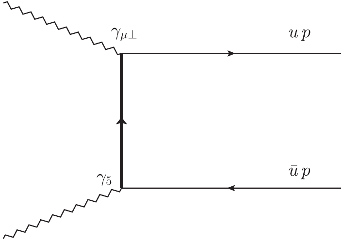
Figure 1. Diagram of leading-order (LO) contribution.
ΠLT,(0)μ(p,q)=−i2ˉn⋅quq2+ˉu(p+q)2−uˉum2ρ−m2Q×ˉq(up)γμ⊥⧸nγ5q(ˉup)=−i2ˉn⋅quq2+ˉu(p+q)2−m2Q×ˉq(up)γμ⊥⧸nγ5q(ˉup)+O(Λ2QCDm2Q).

(8) Using the definition of the leading-twist
ρ DA [28] in Appendix A, we obtain the leading twist tree level factorization formulaΠLT,(0)μ(p,q)=−fTρ(μ)ϵμpqη∫10duϕ⊥(u,μ)1uq2+ˉu(p+q)2−m2Q.

(9) The result (9) can be written in the form of double dispersion relation
ΠLT,(0)μ(p,q)=−fTρ(μ)ϵμpqη∬dsds′×ρLT,(0)(s,s′)[s−q2][s′−(p+q)2],

(10) where the double dispersion density
ρLT,(0) is defined asρLT,(0)(s,s′)=1π2Ims′Ims∫10duϕ⊥(u,μ)us+ˉus′−m2Q.

(11) The expression of wave function
ϕ⊥(u,μ) in terms of Gegenbauer polynomials can be written asϕ⊥(u,μ)=6uˉu∞∑n=0a⊥n(μ)C3/2n(2u−1)=∞∑k=1bkuk,

(12) where
bk is the function of Gegenbauer momentsa(μ) . The spectral density can be obtained as follows [30]ρLT,(0)(t,v)=∞∑k=1bk1π2Ims′Ims∫10duukus+ˉus′−m2Q=∞∑k=1bk(−1)k+1k!12k+1t(m2Qt−ˉv)kδ(k)(v−12)×θ(vt−m2Q).

(13) We defined two variables
t=s+s′,v=ss+s′ in Eq. (13), which are similar to those in our previous study [32].Equating (6) and (10) and applying the double Borel transformation, then subtracting the continuum states using the quark-hadronic duality, we obtain the leading-twist strong coupling constant at LO
gLT,(0)=mQfHfH∗m2HmH∗fTρ(μ)M22ϕ⊥(12,μ)×[em2H+m2H∗−2m2QM2−em2H+m2H∗−2s0M2].

(14) -
The one-loop diagrams are shown in Fig. 2. The loop calculations are similar to those in [32]. We borrow the results from [32] and take the asymptotic form of wave function in Eq. (12) as
ϕ⊥(u)=6uˉu for feasibility of calculation. Subsequently, we adopt a similar procedure to derive the double dispersion spectral densities and apply the double Borel transformation and continuum subtraction to obtain the result. Here, we omit the detailed procedures for simplicity, and the explicit operations with final results are provided in our previous study [32].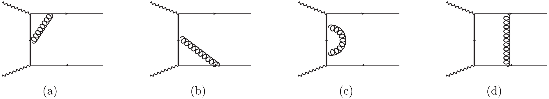
Figure 2. NLO QCD corrections of leading-twist contributions.
Combing the NLO result from [32] with Eq. (14), we obtain the leading-twist sum rules up to
O(αs) , and the coupling constant readsgLT=−mQfHfH∗m2HmH∗em2H+m2H∗M2fTρ(μ)×[−M22ϕ⊥(12,μ)(e−2m2QM2−e−2s0M2)+FLT,(1)],

(15) where
FLT,(1)=αsCF4π{m2Q∫2ˆs0−20dσe−σ+2ˆM2g(σ)+Δg(ˆM2,m2Q)},

(16) and
g(σ)=3Li2(−σ)+3Li2(−σ−1)−6Li2(−σ2)−3lnσ2lnσ+22+3ln(σ+1)ln(σ+2)−6(σ+1)2(σ+2)3ln(σ+1)+3(7σ3+50σ2+100σ+64)4(σ+2)3lnσ2+32lnσ+22+3(11σ2+28σ+24)8(σ+2)2−3lnμ2m2Q−94lnν2μ2−π24,Δg(ˆM2,m2Q)=3(4+3lnμ2m2Q)m2Qe−2m2QM2.

(17) For the scale dependence, we use
ddlnμmQ(μ)=−6αsCF4πmQ(μ),ddlnμfTρ(μ)=−2αsCF4πfTρ(μ),

(18) and we obtain
ddlnμgLT=0+O(α2s),

(19) It is evident that our result is independent of the factorization scale
μ at the one-loop level. -
We perform the subleading power corrections to coupling constants, which are involved with two-particle and three-particle corrections up to twist-4. The higher twist (up to twist-4) Q-quark propagator in the background field is adopted [33]:
⟨0|T{ˉQ(x),Q(0)}|0⟩⊃igs∫d4k(2π)4e−ik⋅x∫10du[uxμk2−m2QGμν(ux)γν−⧸k+mQ2(k2−m2Q)2Gμν(ux)σμν].

(20) For the two-particle corrections, inserting the first term of Eq. (20) into the correlation function (4) and using the DAs of
ρ meson, we gain the higher twist two-particle correctionsΠ2P,HTμ(p,q)=−14ϵμpqη∫10du{−2mQfρmρg(a)⊥(u)+fTρ(μ)m2ρAT(u)[uq2+ˉu(p+q)2−m2Q]2+−2m2QfTρ(μ)m2ρAT(u)[uq2+ˉu(p+q)2−m2Q]3}.

(21) The twist-3
g(a)⊥ corrections are suppressed byO(ΛQCD/mQ) , and twist-4AT corrections are suppressed byO(Λ2QCD/m2Q) compared with the leading-twist corrections (10). To maintain consistency, we must also consider the subleading-power corrections of leading-twist. According to Eq. (8), the correlation function readsΠLT,NLPμ(p,q)=−i2ˉn⋅quˉum2ρ[uq2+ˉu(p+q)2−m2Q]2×ˉq(up)γμ⊥⧸nγ5q(ˉup)=−fTρϵμpqη∫10duϕ⊥(u,μ)×uˉum2ρ[uq2+ˉu(p+q)2−m2Q]2.

(22) Similar to the leading-twist LO case, after applying double Borel transformations and subtracting the continuum states using quark-hadronic duality, we obtain the strong coupling constant for two-particle subleading-power corrections at LO
g2P=−mQfHfH∗m2HmH∗em2H+m2H∗−2m2QM2mρ2[mρ2fTρ(μ)ϕ⊥(12,μ)−mQfρg(a)⊥(12,μ)+mρfTρ(μ)(12+m2QM2)AT(12,μ)].

(23) Considering three-particle corrections at the tree level, the correlation function of the three-particle
qˉqg corrections can be written asΠ3Pμ(p,q)=igs∫d4x∫d4k(2π)4e−i(k+p+q)⋅x×∫10du⟨ρ−(p,η∗)|ˉd(x)γμ⊥[uxαk2−m2Qγβ−⧸k+mQ2(k2−m2Q)2σαβ]Gαβ(ux)γ5q(0)|0⟩.

(24) Employing the conformal expansion of the three-particle DAs in Appendix B, we obtain
g3P=−mQfHfH∗m2HmH∗em2H+m2H∗−2m2QM2fTρ(μ)m2ρ×[(218−4ln2)˜t10(μ)−158s00(μ)].

(25) Collecting Eqs. (15), (23), and (25), the final LCSR reads
gH∗Hρ=−mQfHfH∗m2HmH∗em2H+m2H∗−2m2QM2×{fTρ(μ)[−M22(1−e−2s0−2m2QM2)+m2ρ4]ϕ⊥(12,μ)+fTρ(μ)FLT,(1)e2m2QM2−mQ2mρfρg(a)⊥(12,μ)+m2ρfTρ(μ)[12(12+m2QM2)AT(12,μ)+(218−4ln2)˜t10(μ)−158s00(μ)]},

(26) where
FLT,(1) is defined in Eq. (16). -
The masses of quarks in the
¯MS scheme and the values of decay constants are listed in Table 1. The parameters inρ DAs are listed in Table 2, which are extracted from the method of QCDSR [9,28].¯mc(¯mc) /GeV

¯mb(¯mb) /GeV

fρ /MeV

fTρ(μ0) /MeV

fD /MeV

fD∗ /MeV

fB /MeV

fB∗ /MeV

1.288±0.02 

4.193+0.022−0.035 

213±5 

160±7 

209.0±2.4 

225.3±8.0 

192.0±4.3 

182.4±6.2 

a∥2(μ0) 

a⊥2(μ0) 

ζ3(μ0) 

ωA3(μ0) 

ωV3(μ0) 

ωT3(μ0) 

ζT4(μ0) 

˜ζT4(μ0) 

⟨⟨Q(1)⟩⟩(μ0) 

⟨⟨Q(3)⟩⟩(μ0) 

⟨⟨Q(5)⟩⟩(μ0) 

0.17±0.07 

0.14±0.06 

0.032±0.010 

−2.1±1.0 

3.8±1.8 

7.0±7.0 

0.10±0.05 

−0.10±0.05 

−0.15±0.15 

0 

0 

Table 2. Non-perturbative parameters in DAs at scale
μ0=1.0GeV. The solution to the two-loop evolution of the Gegenbauer moment
a⊥n(μ) isfTρ(μ)a⊥n(μ)=[ENLOT,n(μ,μ0)+αs(μ)4πn−2∑k=0ELOT,n(μ,μ0)×dkT,n(μ,μ0)]fTρ(μ0)a⊥n(μ0),

(27) where the explicit expressions of
ET,n anddT,n can be found in [39]. The scale evolution of other non-perturbative parameters to leading logarithmic accuracy is listed in Appendix B.The factorization scales are taken as
μc∈[1,2] GeV around the default choicemc andμb=mb+mb−mb/2 for radiativeD∗ andB∗ decays, respectively. For the Borel massM2 and the threshold parameters0 , we assume the following intervals [40,41]{s0=6.0±0.5GeV2,M2=4.5±1.0GeV2,forD∗Dρ;{s0=34.0±1.0GeV2,M2=18.0±3.0GeV2,forB∗Bρ,

(28) which satisfy the standard criterions [42].
-
The coupling constants for
D∗Dρ andB∗Bρ are listed in Table 3. It is apparent that the perturbative QCD corrections decrease the tree level leading power contributions of coupling constants by 10% and 20% forD∗Dρ andB∗Bρ , respectively. Meanwhile, contributions from tree level sub-leading power corrections have evident compensation effects, which increase the leading twist contributions by approximately 20% and 30% forD∗Dρ andB∗Bρ , respectively. We also note that three-particle sub-leading power corrections have more minor effects compared with two-particle sub-leading power corrections, particularly for the coupling ofB∗Bρ , which is consistent with the validity of OPE.gLT,LL 

gLT,NLL 

g2P,LL 

g3P,LL 

Total D∗Dρ 

3.61+0.54−0.47 

3.18+0.53−0.43 

0.47+0.17−0.16 

0.14+0.09−0.08 

3.80+0.59−0.45 

B∗Bρ 

3.59+0.55−0.43 

2.91+0.38−0.42 

0.96+0.23−0.15 

0.022+0.013−0.012 

3.89+0.52−0.48 

Table 3. Results of
gH∗Hρ (GeV−1 ).gLT,LL corresponds to the tree-level leading power contributions with resummation at LL accuracy;gLT,NLL corresponds to the leading power contributions up to NLO with resummation at NLL accuracy;g2P,LL andg3P,LL are from 2-particle and 3-particle sub-leading power corrections at LO separately.The uncertainties are also included for separate terms of coupling constants in Table 3. The uncertainties are estimated by varying independent input parameters, and the individual uncertainties are presented in Table 4. To estimate total uncertainties, we add them in quadrature to obtain the final results. From Table 4, we can see that the primary uncertainties stem from the Borel mass
M2 and parametera⊥2 both forD∗Dρ andB∗Bρ . The second Gegenbauer momenta⊥2 refers to transversely polarizedρ meso twist-4 LCDA, which is indicated in Appendix A, B. The quasi-distribution amplitudes (quasi-DAs), which are based on the large-momentum effective theory (LaMET) [43,44], along with the simulation from lattice QCD [45] are also capable of extracting meson LCDA [46,47] other than QCDSR. In the future, a more precise determination of theρ meson LCDA will be helpful to decrease the uncertainties of couplings.Central value ΔfH∗ 

ΔmQ 

ΔM2 

Δμ 

ΔfTρ 

Δa⊥2 

gD∗Dρ 

3.80+0.50−0.45 

+0.14−0.13 

+0.00−0.01 

+0.38−0.20 

+0.20−0.01 

±0.11 

±0.32 

gB∗Bρ 

3.89+0.52−0.48 

+0.14−0.13 

+0.12−0.08 

+0.36−0.23 

+0.14−0.26 

±0.12 

±0.24 

Table 4. Central value and individual uncertainty of
gH∗Hρ (GeV−1 ) due to variations in input parameters. We only list numerically significant uncertainties.Next, we compare our results of coupling constants with those obtained in other studies using sum rules, as shown in Table 5. Among them, the LCSR studies [24,26] did not take the perturbative QCD corrections and 3-particle corrections into account, and the QCDSR study considers the dimension-5 quark-gluon condensate corrections [29]. As mentioned above, the NLO effects of leading power almost cancel the subleading-power corrections; hence, it is expected that our results are close to those of previous sum rules studies within the errors.
Table 5. Numerical values of coupling constants
gH∗Hρ (GeV−1 ) from several studies via sum rules.Next, we extract the
B∗Bρ coupling from form factors. TheB→ρ form factorsV(q2) andT1(q2) , which are related togB∗Bρ , are defined as⟨ρ−(p,η∗)|ˉdγμb|B−(p+q)⟩=2mB+mρV(q2)ϵμηpq,⟨ρ−(p,η∗)|ˉdiσμνqνb|B−(p+q)⟩=−2T1(q2)ϵμηpq.

(29) From the dispersion relation of the form factor
Fi(q2) Fi(q2)=ri11−q2/m2B∗+∫∞(mB+mρ)2ρ(s)s−q2−iϵ,

(30) the strong coupling relates to the pole of the form factors at the unphysical point
q2=m2B∗ . Then, we have the relationrV1=lim

(31) where
f_{B^*}^T is the tensor coupling of theB^* meson, and it is defined as\begin{array}{l} \langle\,0\,|\,\bar{b}\,\sigma_{\mu\nu}\,q\,|\,B^*(q,\epsilon)\,\rangle = {\rm i}\,f_{B^*}^T\,(\epsilon_\mu\,q_\nu-\epsilon_\nu\,q_\mu)\,. \end{array}

(32) Using Eq. (31) and choosing the size
f_{B^*}^T = f_{B^*} , we extract several numerical values of the couplingg_{B^*B\rho} from recent LCSR studies [9,10], which we list in Table 6.Table 6. Coupling
g_{B^*B\rho} (\rm{GeV}^{-1} ) from the residue ofB\to\rho form factor V andT_1 in LCSR fit and compared to our result.As shown, our central value is smaller than the extrapolations from LCSR form factors. To explain this discrepancy, on the one hand, uncertainties from the parameterizations of form factors to obtain the un-physical singularity may be underestimated. On the other hand, for the double dispersion relation, the Borel suppression is not sufficient to neglect the isolated excitation contributions, according to the discussion in [48]. Apart from
B \to \rho , theB^* \to B andB^* \to \rho form factors can also be used to extract the coupling. To the best of our knowledge, there are no relevant studies that address corresponding form factors in LCSR. A future study could verify whether different choices of form factors are consistent across the coupling extractions.Finally, we analyze our study and compare it with other model-dependent studies. The HM
\chi PT effective Lagrangian to parametrize theH^*HV coupling can be written as [1]\begin{array}{l} {\cal{L}}_V = {\rm i}\,\lambda\,{\rm Tr}[{\cal{H}}_b\,\sigma^{\mu\nu}\,F_{\mu\nu}(\rho)_{ba}\,\bar{{\cal{H}}}_a]\,, \end{array}

(33) with
\begin{array}{l} F_{\mu\nu}(\rho) = \partial_\mu\, \rho_\nu-\partial_\nu\, \rho_\mu +[\rho_\mu,\,\rho_\nu]\,, \quad \rho_\mu = {\rm i}\,\dfrac{g_V}{\sqrt{2}}\,\hat{\rho}_\mu\,, \end{array}

(34) where
\hat{\rho} is a3\times 3 matrix for light meson nonet, and the heavyH, H^* mesons are represented by the doublet field{\cal{H}}_a with the conventional normalization. The parameterg_V = m_\rho/f_\pi . In the chiral and heavy quark limits, we have the following relation for the coupling\lambda \begin{array}{l} \lambda = \dfrac{\sqrt{2}}{4}\,\dfrac{1}{g_V}\,g_{H^*H\rho}\,. \end{array}

(35) We find the coupling
\lambda = 0.23\pm0.03\,{\rm GeV}^{-1} at leading power from our value ofg_{B^*B\rho} .In Table 7, we compare this value with other model estimations. Similar to the estimations from form factors, our result is smaller than the model predictions.
Table 7. Central value of coupling
\lambda (\rm{GeV}^{-1} ) from model estimations compared to our result.One possibility for this discrepancy may be that the model predictions have potentially larger errors. Consequently, in principle, the LCSR is more credible. However, in addition to the possible influences of excitation contributions mentioned above, the values of NLO corrections to higher twists and the sub-sub-leading power contributions are unknown, which may likewise represent sources of the discrepancy. Improvements in the calculations of both the sum rules and models may help better understand such discrepancies in the future.
-
We compute the
D^*D\rho andB^*B\rho strong couplings to subleading-power in LCSR. Long-distance dynamics are incorporated in the\rho DAs. We calculate the{\cal{O}}(\alpha_s) corrections to leading power of the sum rules. The subleading-power corrections are calculated at LO by accounting the two- and three-particle wave functions up to twist-4. The analytical results of the double spectral densities are obtained, and in accordance with the previous study, we also perform a continuum subtraction for the higher-twist corrections. The LO results are independent of the choice of the duality region because of the special form of the double spectral density.The NLO corrections reduce the numerical tree-level results by 10% and 20% for
D^*D\rho andB^*B\rho , respectively. However, the subleading-power corrections at LO can give rise to values about 20% and 30% forD^*D\rho andB^*B\rho , respectively. Summing all the contributions, our values are consistent with the predictions from previous sum rules studies. Moreover, we also predict the coupling\lambda in HM\chi PT at leading power. The central value of our result is smaller than the existing model-dependent estimations. Possible explanations for the discrepancy are potentially large errors within models and influences of excitation contributions in LCSR. Moreover, radiative corrections to higher twists and sub-sub-leading power contributions may also be sources of error. A better understanding of this discrepancy will prove beneficial to shedding light on long-distance QCD dynamics in the future.We are grateful to Prof. Cai-dian Lü and Prof. Yue-long Shen for helpful discussions.
-
Here, we collect the
\rho meson DAs up to twist-4, which are defined in [28]\tag{A1}\begin{split} \langle\,\rho^-(p,\eta^*)\,|\,\bar{d}(x)\,\gamma_\mu\,u(0)\,|\,0\,\rangle = \; f_\rho\,m_\rho\,\bigg\{\frac{\eta^*\cdot x}{p\cdot x}\,p_\mu\int_0^1{\rm d}u\,{\rm e}^{{\rm i}\,u\,p\cdot x}\,\big[\phi_\parallel(u)+\frac{m_\rho^2\,x^2}{16}\,\mathbb{A}(u)\big] +\eta^*_{\perp\mu}\int_0^1{\rm d}u\,{\rm e}^{{\rm i}\,u\,p\cdot x}\,g_\perp^{(v)}(u)-\frac{1}{2}\,x_\mu\,\frac{\eta^*\cdot x}{(p\cdot x)^2}\,m_\rho^2 \int_0^1{\rm d}u\,{\rm e}^{{\rm i}\,u\,p\cdot x}\,g_3(u)\bigg\}\,, \end{split}

(A1) \tag{A2} \begin{split} \langle\,\rho^-(p,\eta^*)\,|\,\bar{d}(x)\,\gamma_\mu\,\gamma_5\,u(0)\,|\,0\,\rangle = \frac{1}{4}\,f_\rho\,m_\rho\,\epsilon_{\mu\eta px} \int_0^1{\rm d}u\,{\rm e}^{{\rm i}\,u\,p\cdot x}\,g_\perp^{(a)}(u)\,, \end{split}

(A2) \tag{A3} \begin{split} \langle\,\rho^-(p,\eta^*)\,|\,\bar{d}(x)\,\sigma_{\mu\nu}\,u(0)\,|\,0\,\rangle =& -{\rm i}\,f_\rho^T\,\bigg\{ (\eta^*_{\perp\mu}\,p_\nu-\eta^*_{\perp\nu}\,p_\mu) \int_0^1{\rm d}u\,{\rm e}^{{\rm i}\,u\,p\cdot x}\, \big[\phi_\perp(u)+\frac{m_\rho^2\,x^2}{16}\,\mathbb{A}_T(u)\big] +(p_\mu\,x_\nu-p_\nu\,x_\mu)\,\frac{\eta^*\cdot x}{(p\cdot x)^2}\,m_\rho^2 \int_0^1{\rm d}u\,{\rm e}^{{\rm i}\,u\,p\cdot x}\,h_\parallel^{(t)}(u) \\ &+\frac{1}{2}\,\frac{\eta^*_{\perp\mu}\,x_\nu-\eta^*_{\perp\nu}\,x_\mu}{p\cdot x}\,m_\rho^2 \int_0^1{\rm d}u\,{\rm e}^{{\rm i}\,u\,p\cdot x}\,h_3(u) \bigg\}\,, \end{split}

(A3) \tag{A4} \begin{split} \langle\,\,\rho^-(p,\eta^*)\,|\,\bar{d}(x)\,u(0)\,|\,0\,\rangle = -\frac{\rm i}{2}\,f_\rho^T\,(\eta^*\cdot x) \,m_\rho^2 \int_0^1{\rm d}u\,{\rm e}^{{\rm i}\,u\,p\cdot x}\,h_\parallel^{(s)}(u)\,, \end{split}

(A4) \tag{A5}\begin{split} \langle\,\rho^-(p,\eta^*)\,|\,\bar{d}(x)\,g_s\,\tilde{G}_{\mu\nu}(vx)\,\gamma_\alpha\,\gamma_5\,u(0)\,|\,0\,\rangle =& -f_\rho\,m_\rho\,p_\alpha\,\big[p_\nu\, \eta^*_{\perp\mu}-p_\mu\,\eta^*_{\perp\nu}\big]\int[D\alpha]\,{\rm e}^{{\rm i}\,(\alpha_q+v\,\alpha_g)\,p\cdot x}\,{\cal{A}}(\alpha) -f_\rho\,m_\rho^3\,\frac{\eta^*\cdot x}{p\cdot x}\,\big[p_\mu\,g^\perp_{\alpha\nu}-p_\nu\,g^\perp_{\alpha\mu}\big] \\ &\times\int[D\alpha]\,{\rm e}^{{\rm i}\,(\alpha_q+v\,\alpha_g)\,p\cdot x}\,\tilde{\Phi}(\alpha) -f_\rho\,m_\rho^3\,\frac{\eta^*\cdot x}{(p\cdot x)^2}\, p_\alpha\, \big[p_\mu\,x_\nu-p_\nu\,x_\mu\big]\int[D\alpha]\,{\rm e}^{{\rm i}\,(\alpha_q+v\,\alpha_g)\,p\cdot x}\, \tilde{\Psi}(\alpha)\,, \end{split}

(A5) \tag{A6} \begin{split} \langle\,\rho^-(p,\eta^*)\,|\,\bar{d}(x)\,g_s\,G_{\mu\nu}(vx)\,i\,\gamma_\alpha\,u(0)\,|\,0\,\rangle =& -f_\rho\,m_\rho\,p_\alpha\,\big[p_\nu\, \eta^*_{\perp\mu}-p_\mu\,\eta^*_{\perp\nu}\big]\int[D\alpha]\,{\rm e}^{{\rm i}\,(\alpha_q+v\,\alpha_g)\,p\cdot x}\,{\cal{V}}(\alpha) -f_\rho\,m_\rho^3\,\frac{\eta^*\cdot x}{p\cdot x}\,\big[p_\mu\,g^\perp_{\alpha\nu}-p_\nu\,g^\perp_{\alpha\mu}\big] \\ &\times\int[D\alpha]\,{\rm e}^{{\rm i}\,(\alpha_q+v\,\alpha_g)\,p\cdot x}\,\Phi(\alpha) -f_\rho\,m_\rho^3\,\frac{\eta^*\cdot x}{(p\cdot x)^2}\, p_\alpha\, \big[p_\mu\,x_\nu-p_\nu\,x_\mu\big]\int[D\alpha]\,{\rm e}^{{\rm i}\,(\alpha_q+v\,\alpha_g)\,p\cdot x}\,\Psi(\alpha)\,, \end{split}

(A6) \tag{A7} \begin{split} \langle\,\rho^-(p,\eta^*)\,|\,\bar{d}(x)\,g_s\,G_{\mu\nu}(vx)\,\sigma_{\alpha\beta}\,u(0)\,|\,0\,\rangle = & f^T_\rho\,m_\rho^2\,\frac{\eta^*\cdot x}{2\,p\cdot x} \,\big[ p_\alpha\,p_\mu\,g^\perp_{\beta\nu}-p_\beta\,p_\mu\,g^\perp_{\alpha\nu}-(\mu\leftrightarrow \nu) \big] \int[D\alpha]\,{\rm e}^{{\rm i}\,(\alpha_q+v\,\alpha_g)\,p\cdot x}\,{\cal{T}}(\alpha) +f^T_\rho\,m_\rho^2\,\big[ p_\alpha\,\eta^*_{\perp\mu}\,g^\perp_{\beta\nu}-p_\beta\,\eta^*_{\perp\mu} \,g^\perp_{\alpha\nu}-(\mu\leftrightarrow \nu) \big]\\&\times \int[D\alpha]\,{\rm e}^{{\rm i}\,(\alpha_q+v\,\alpha_g)\,p\cdot x}\,T_1^{(4)}(\alpha) +f^T_\rho\,m_\rho^2\,\big[ p_\mu\,\eta^*_{\perp\alpha}\,g^\perp_{\beta\nu}-p_\mu\,\eta^*_{\perp\beta} \,g^\perp_{\alpha\nu} -(\mu\leftrightarrow \nu) \big] \int[D\alpha]\,{\rm e}^{{\rm i}\,(\alpha_q+v\,\alpha_g)\,p\cdot x}\,T_2^{(4)}(\alpha)\\& +f^T_\rho\,m_\rho^2\,\frac{(p_\mu\,x_\nu-p_\nu\,x_\mu)\,(p_\alpha\,\eta^*_{\perp\beta}-p_\beta\,\eta^*_{\perp\alpha})}{p\cdot x} \int[D\alpha]\,{\rm e}^{{\rm i}\,(\alpha_q+v\,\alpha_g)\,p\cdot x}\,T_3^{(4)}(\alpha)\\& +f^T_\rho\,m_\rho^2\,\frac{(p_\alpha\,x_\beta-p_\beta\,x_\alpha)\,(p_\mu\,\eta^*_{\perp\nu}-p_\nu\,\eta^*_{\perp\mu})}{p\cdot x} \int[D\alpha]\,{\rm e}^{{\rm i}\,(\alpha_q+v\,\alpha_g)\,p\cdot x}\,T_4^{(4)}(\alpha)\,, \\[-13pt]\end{split}

(A7) \tag{A8} \begin{split} \langle\,\rho^-(p,\eta^*)\,|\,\bar{d}(x)\,g_s\,G_{\mu\nu}(vx)\,u(0)\,|\,0\,\rangle = -{\rm i}\,f^T_\rho\,m_\rho^2\,\big[\eta^*_{\perp\mu}\,p_\nu-\eta^*_{\perp\nu}\,p_\mu\big]\int[D\alpha]\,{\rm e}^{{\rm i}\,(\alpha_q+v\,\alpha_g)\,p\cdot x}\,S(\alpha)\,, \end{split}

(A8) \tag{A9}\begin{split} \langle\,\rho^-(p,\eta^*)\,|\,\bar{d}(x)\,{\rm i}\,g_s\,\tilde{G}_{\mu\nu}(vx)\,\gamma_5\,u(0)\,|\,0\,\rangle = {\rm i}\,f^T_\rho\,m_\rho^2\,\big[\eta^*_{\perp\mu}\,p_\nu-\eta^*_{\perp\nu}\,p_\mu\big]\int[D\alpha]\,{\rm e}^{{\rm i}\,(\alpha_q+v\,\alpha_g)\,p\cdot x}\,\tilde{S}(\alpha)\,, \end{split}

(A9) where
\tag{A10} \begin{split} \widetilde{G}_{\alpha \beta} = \frac{1}{2} \, \epsilon_{\alpha \beta \rho \tau } \, G^{\rho \tau} \,. \end{split}

(A10) -
Here, we list the conformal expansion for these higher twist DAs involved in our calculation [28].
The chiral-even twist-three DA
g_\perp^{(a)} reads\tag{B1} \begin{split} g_\perp^{(a)}(u) = 6\,u\,\bar{u}\,\Big\{1+ \Big[\frac{1}{4}\,a_2^\parallel +\frac{5}{3}\,\zeta_3\,\Big(1-\frac{3}{16}\,\omega_3^A +\frac{9}{16}\,\omega_3^V\Big)\Big] \,(5\,\xi^2-1) \Big\}\,, \end{split}

(B1) with
\xi = 2\,u-1 . For the chiral-odd twist-four DA\mathbb{A}_T , we have\tag{B2} \begin{split} \mathbb{A}_T(u) =& 30\,u^2\,\bar{u}^2\,\Big[\frac{2}{5}\,\Big(1+\frac{2}{7}\,a_2^\perp+ \frac{10}{3}\,\zeta_4^T- \frac{20}{3}\,\tilde{\zeta}_4^T\Big)\\&+\Big(\frac{3}{35}\,a_2^\perp+\frac{1}{40}\,\zeta_3\,\omega_3^T\Big)\,C_2^{5/2}(\xi)\Big] \\& -\Big[\frac{18}{11}\,a_2^\perp-\frac{3}{2}\,\zeta_3\,\omega_3^T+ \frac{126}{55}\,\langle\langle Q^{(1)}\rangle\rangle \\&+\frac{70}{11}\,\langle\langle Q^{(3)}\rangle\rangle\Big]\, \big[u\,\bar{u}\,(2+13\,u\,\bar{u}) \\& +2\,u^3\,(10-15\,u+6\,u^2)\,\ln u \\&+2\,\bar{u}^3\,(10-15\,\bar{u}+6\,\bar{u}^2)\,\ln \bar{u}\big]\,. \end{split}

(B2) For the twist-4 three-particle DAs,
\begin{split} S(\alpha_i) =& \; 30\,\alpha_g^2\,\Big\{ s_{00}\,(1-\alpha_g)+s_{10}\, \Big[ \alpha_g\,(1-\alpha_g)-\frac{3}{2}\,(\alpha_{\bar{q}}^2+ \alpha_q^2) \Big] \\ & +s_{01}\, \big[ \alpha_g\,(1-\alpha_g)-6\,\alpha_{\bar{q}}\,\alpha_q \big]\Big\}\,, \\ \tilde{S}(\alpha_i) =& \; 30\,\alpha_g^2\,\Big\{ \tilde{s}_{00}\,(1-\alpha_g)+\tilde{s}_{10}\, \Big[ \alpha_g\,(1-\alpha_g)-\frac{3}{2}\,(\alpha_{\bar{q}}^2+ \alpha_q^2) \Big] \\ & +\tilde{s}_{01}\, \big[ \alpha_g\,(1-\alpha_g)-6\,\alpha_{\bar{q}}\,\alpha_q \big]\Big\}\,, \\ T_1^{(4)}(\alpha_i) =& \; 120\,t_{10}\,(\alpha_{\bar{q}}-\alpha_q)\, \alpha_{\bar{q}}\,\alpha_q\,\alpha_g\,, \\ T_2^{(4)}(\alpha_i) =& -30\,\alpha_g^2\,(\alpha_{\bar{q}}-\alpha_q)\, \Big[\tilde{s}_{00}+\frac{1}{2}\, \tilde{s}_{10}\, (5\,\alpha_g-3)+\tilde{s}_{01}\,\alpha_g\Big]\,, \\\end{split}

(B3) \tag{B3} \begin{split} T_3^{(4)}(\alpha_i) =& -120\,\tilde{t}_{10}\,(\alpha_{\bar{q}}-\alpha_q)\, \alpha_{\bar{q}}\,\alpha_q\,\alpha_g\,, \\ T_4^{(4)}(\alpha_i) =& \; 30\,\alpha_g^2\,(\alpha_{\bar{q}}-\alpha_q)\, \Big[s_{00}+\frac{1}{2}\, s_{10}\, (5\,\alpha_g-3) +s_{01}\,\alpha_g\Big]\,. \end{split}

(B3) The eight parameters in three-particle DAs can be written as
\tag{B4} \begin{split} s_{00} =& \zeta_4^T\,\quad \tilde{s}_{00} = \tilde{\zeta}_4^T\,, \\ s_{10} =& -\frac{3}{22}\,a_2^\perp-\frac{1}{8}\,\zeta_3\,\omega_3^T+\frac{28}{55}\,\langle\langle Q^{(1)}\rangle\rangle +\frac{7}{11}\,\langle\langle Q^{(3)}\rangle\rangle+ \frac{14}{3}\,\langle\langle Q^{(5)}\rangle\rangle\,, \\ \tilde{s}_{10} =& \frac{3}{22}\,a_2^\perp-\frac{1}{8}\,\zeta_3\,\omega_3^T-\frac{28}{55}\,\langle\langle Q^{(1)}\rangle\rangle -\frac{7}{11}\,\langle\langle Q^{(3)}\rangle\rangle+ \frac{14}{3}\,\langle\langle Q^{(5)}\rangle\rangle\,, \\ s_{01} =& \frac{3}{44}\,a_2^\perp+\frac{1}{8}\,\zeta_3\,\omega_3^T+\frac{49}{110}\,\langle\langle Q^{(1)}\rangle\rangle -\frac{7}{22}\,\langle\langle Q^{(3)}\rangle\rangle+ \frac{7}{3}\,\langle\langle Q^{(5)}\rangle\rangle\,, \\ \tilde{s}_{01} =& -\frac{3}{44}\,a_2^\perp+\frac{1}{8}\,\zeta_3\,\omega_3^T-\frac{49}{110}\,\langle\langle Q^{(1)}\rangle\rangle +\frac{7}{22}\,\langle\langle Q^{(3)}\rangle\rangle+ \frac{7}{3}\,\langle\langle Q^{(5)}\rangle\rangle\,, \\ t_{10} =& -\frac{9}{44}\,a_2^\perp-\frac{3}{16}\,\zeta_3\,\omega_3^T-\frac{63}{220}\,\langle\langle Q^{(1)}\rangle\rangle +\frac{119}{44}\,\langle\langle Q^{(3)}\rangle\rangle\,, \\ \tilde{t}_{10} =& \frac{9}{44}\,a_2^\perp-\frac{3}{16}\,\zeta_3\,\omega_3^T+\frac{63}{220}\,\langle\langle Q^{(1)}\rangle\rangle +\frac{35}{44}\,\langle\langle Q^{(3)}\rangle\rangle\,. \end{split}

(B4) The scale evolution of non-perturbative parameters to leading logarithmic accuracy is as follows
\tag{B5}\begin{split} a_{2}^{\parallel }(\mu )=&{{L}^{\frac{25}{6}{{C}_{F}}/{{\beta }_{0}}}}a_{2}^{\parallel }({{\mu }_{0}}), \\{{\zeta }_{3}}(\mu )=&{{L}^{\left( -\frac{1}{3}{{C}_{F}}+3{{C}_{A}} \right)/{{\beta }_{0}}}}{{\zeta }_{3}}({{\mu }_{0}}), \\ \omega _{3}^{T}(\mu )=&{{L}^{\left( \frac{25}{6}{{C}_{F}}-2{{C}_{A}} \right)/{{\beta }_{0}}}}\omega _{3}^{T}({{\mu }_{0}}), \\ (\zeta _{4}^{T}+\tilde{\zeta }_{4}^{T})(\mu )=&{{L}^{\left( 3{{C}_{A}}-\frac{8}{3}{{C}_{F}} \right)/{{\beta }_{0}}}}(\zeta _{4}^{T}+\tilde{\zeta }_{4}^{T})({{\mu }_{0}}), \\ (\zeta _{4}^{T}-\tilde{\zeta }_{4}^{T})(\mu )=&{{L}^{\left( 4{{C}_{A}}-4{{C}_{F}} \right)/{{\beta }_{0}}}}(\zeta _{4}^{T}-\tilde{\zeta }_{4}^{T})({{\mu }_{0}}), \\ \langle \langle {{Q}^{(1)}}\rangle \rangle (\mu )=&{{L}^{\left( -4{{C}_{F}}+\frac{11}{2}{{C}_{A}} \right)/{{\beta }_{0}}}}\langle \langle {{Q}^{(1)}}\rangle \rangle ({{\mu }_{0}}), \\ \langle \langle {{Q}^{(3)}}\rangle \rangle (\mu )=&{{L}^{\frac{10}{3}{{C}_{F}}/{{\beta }_{0}}}}\langle \langle {{Q}^{(3)}}\rangle \rangle ({{\mu }_{0}}), \\\langle \langle {{Q}^{(5)}}\rangle \rangle (\mu )=&{{L}^{\left( -\frac{5}{3}{{C}_{F}}+5{{C}_{A}} \right)/{{\beta }_{0}}}}\langle \langle {{Q}^{(5)}}\rangle \rangle ({{\mu }_{0}}), \\ \end{split}

(B5) where
L = \alpha_s(\mu)/\alpha_s(\mu_0) and\beta_0 = 11-2\,n_f/3 ,n_f being the number of flavors involved. The scale-dependence of\omega^{V(A)}_\gamma(\mu) \tag{B6} \begin{split} \left( \begin{array}{c} \omega^{V}_3(\mu) - \omega^{A}_3(\mu) \\ \omega^{V}_3(\mu) + \omega^{A}_3(\mu) \end{array} \right) = L^{\Gamma_{\omega} / \beta_0} \, \left( \begin{array}{c} \omega^{V}_3(\mu_0) - \omega^{A}_3(\mu_0) \\ \omega^{V}_3(\mu_0) + \omega^{A}_3(\mu_0) \end{array} \right) \,, \end{split}

(B6) where
\Gamma_{\omega} is given by\tag{B7} \begin{split} \Gamma_{\omega} = \left( \begin{array}{c} 3 \, C_F - {2 \over 3} \, C_A \qquad {2 \over 3} \, C_F - {2 \over 3} \, C_A \\ {5 \over 3} \, C_F - {4 \over 3} \, C_A \qquad {1 \over 2} \, C_F + C_A \end{array} \right)\,. \end{split}

(B7)
D*Dρ and B*Bρ strong couplings in light-cone sum rules
- Received Date: 2020-02-15
- Available Online: 2020-07-01
Abstract: We present an improved calculation of the strong coupling constants


 DownLoad: